11.4 BO for Materials Discovery¶

Simple-regret curves versus number of evaluations comparing Bayesian optimisation with Expected Improvement against random search, averaged over 30 seeds, with the BO curve dropping roughly an order of magnitude faster — Figure 11.4.1. Simple-regret curves for Bayesian optimisation (EI) versus random search on a synthetic benchmark, averaged over 30 random seeds. BO converges roughly an order of magnitude faster on this problem — the same advantage typically seen on real materials-discovery tasks where each evaluation is expensive.

Sections 11.1–11.3 built the Bayesian optimisation machinery in the abstract. This section connects it to materials. The questions we must answer to apply BO to a real campaign are practical and unglamorous. What does a candidate material look like as a numerical vector? What counts as the oracle, and how expensive is it? How do we wire all of this together into a campaign that interleaves prediction, querying and update? Two case studies — perovskite band-gap optimisation and catalyst screening with BoTorch — provide the structure; the broader discussion treats featurisation, multi-fidelity coupling, and autonomous experimentation.

Key Idea (Box 11.4.A)

Applying BO to a real materials campaign requires three concrete choices on top of the abstract machinery: (i) a featurisation that maps each candidate material to a numerical vector, (ii) an oracle that evaluates candidates with some accuracy and cost, and (iii) a workflow that closes the loop in software. The mathematical part (GP + EI) is the easy bit; getting these three choices right is what separates a working campaign from a frustrating one.

11.4.1 Featurising a material for BO¶

Bayesian optimisation operates on a continuous input space — the GP kernel needs to compute distances between inputs. A material, however, is naturally described by a discrete chemical formula and an arrangement of atoms in a unit cell. Bridging these two views is the featurisation problem.

Three approaches dominate.

Compositional descriptors. Encode each material by a fixed-length vector summarising its composition. The Magpie set of Ward et al. (2016) is the workhorse: 132 features computed by taking weighted averages and ranges of elemental properties (atomic number, electronegativity, group, period, atomic radius, etc.) over the constituent elements.

Worked Magpie features for Fe$_2$O$_3$

With stoichiometry $(x_\mathrm{Fe}, x_\mathrm{O}) = (0.4, 0.6)$ and elemental properties $Z_\mathrm{Fe} = 26, Z_\mathrm{O} = 8$, $\chi_\mathrm{Fe} = 1.83, \chi_\mathrm{O} = 3.44$ (Pauling electronegativity), the Magpie weighted mean atomic number is $0.4 \cdot 26 + 0.6 \cdot 8 = 15.2$. The weighted mean electronegativity is $0.4 \cdot 1.83 + 0.6 \cdot 3.44 = 2.80$. The electronegativity range is $3.44 - 1.83 = 1.61$. Continuing across the 132 features yields a vector that summarises the composition's elemental properties. Two oxides with similar Magpie vectors are chemically similar in this aggregate sense — useful for a GP kernel. For a binary oxide A$_x$B$_y$O$_z$, the Magpie

features summarise the elemental properties of A and B weighted by their stoichiometry. Magpie features are cheap, deterministic, and respect the natural smoothness of composition space — small changes in stoichiometry produce small changes in the feature vector.

Structural descriptors. When the structure (not just composition) matters, we need descriptors like SOAP, ACSF, or pre-trained GNN embeddings (Chapter 9, Chapter 10). These capture atomic neighbourhoods directly but can be high-dimensional. For BO with a GP, high-dimensional features are problematic — the curse of dimensionality bites — so one typically projects to 50–100 dimensions via PCA or learns a low-dimensional embedding.

Learned latent features. Train a property-prediction GNN (Chapter 10) on a large database, then use the last hidden layer's activations as a fixed feature for BO. The features are tailored to the property of interest, dense, and typically 64–256-dimensional. The cost is training the GNN once upfront; the benefit is featurisation quality that no hand-crafted descriptor can match. This is the modern default.

For one-off campaigns with small candidate sets ($\lesssim 10^3$), Magpie features and an RBF-kernel GP work well. For larger campaigns or for problems where structure-property relationships dominate, GNN embeddings are worth the upfront training cost.

Pause and recall

Before reading on, try to answer these from memory:

Why does a material need to be featurised before Bayesian optimisation can be applied to it?
Name the three dominant featurisation approaches, and state one situation where each is the natural choice.
Beyond the abstract GP-plus-acquisition machinery, what are the three concrete choices that turn BO into a working materials campaign?

If any of these is shaky, re-read the preceding section before continuing.

11.4.2 Case study 1: perovskite band-gap optimisation¶

The first case study is a stylised but realistic problem. We have a library of cubic perovskite candidates ABX$_3$ with $A \in \{$Cs, Rb, K, Na, MA$\}$ (MA = methylammonium), $B \in \{$Pb, Sn, Ge$\}$, $X \in \{$I, Br, Cl$\}$, giving $5 \times 3 \times 3 = 45$ candidates. Each candidate's "true" band gap is, in our simulation, a known function returned by a hypothetical DFT calculation. The goal is to find the candidate with band gap closest to 1.4 eV (the Shockley–Queisser optimum for solar cells) while running as few DFT calculations as possible.

We featurise each candidate via Magpie:

from __future__ import annotations

import itertools

import numpy as np
from matminer.featurizers.composition import ElementProperty
from pymatgen.core import Composition


A_set = ["Cs", "Rb", "K", "Na", "C N H6"]  # methylammonium proxy
B_set = ["Pb", "Sn", "Ge"]
X_set = ["I", "Br", "Cl"]

featuriser = ElementProperty.from_preset("magpie")

candidates: list[dict] = []
for A, B, X in itertools.product(A_set, B_set, X_set):
    formula = f"({A})({B})({X})3"
    comp = Composition(formula)
    features = featuriser.featurize(comp)
    candidates.append({"A": A, "B": B, "X": X, "features": np.array(features)})

X_all = np.vstack([c["features"] for c in candidates])  # (45, 132)

# Standardise.
mean = X_all.mean(axis=0)
std = X_all.std(axis=0) + 1e-8
X_all = (X_all - mean) / std

For the simulated objective we use a smooth function of three chemical proxies — average ionic radius, Pauling electronegativity difference and electron affinity — designed so the minimum-gap-error candidate lies near MA-Pb-I (the real-world champion lead-halide perovskite, which has gap $\sim 1.55$ eV).

def simulated_band_gap(features: np.ndarray) -> float:
    # Some smooth function of the standardised features.
    # In reality this would call DFT or an MLIP.
    rng_global = np.random.default_rng(13)
    coefs = rng_global.normal(0, 1, size=features.shape[0])
    return float(0.7 * np.sin(features @ coefs / 8) + 1.5)


def gap_error(features: np.ndarray) -> float:
    """Distance from the target band gap of 1.4 eV."""
    return -abs(simulated_band_gap(features) - 1.4)

We negate the gap error so the BO objective is to maximise $-|\mathrm{gap} - 1.4|$, which puts the optimum at gap exactly 1.4 eV.

The BO loop, using our GP from §11.2 and EI from §11.3:

# Initialise with three random candidates.
rng = np.random.default_rng(42)
seen_idx = list(rng.choice(45, size=3, replace=False))
remaining_idx = [i for i in range(45) if i not in seen_idx]

X_train = X_all[seen_idx]
y_train = np.array([gap_error(X_all[i]) for i in seen_idx])

history = list(y_train.copy())

for iteration in range(15):
    gp = GP()
    gp.optimise_hyperparameters(X_train, y_train)
    X_remaining = X_all[remaining_idx]
    ei = expected_improvement(gp, X_remaining, float(np.max(y_train)), xi=0.01)
    next_local_idx = int(np.argmax(ei))
    next_global_idx = remaining_idx[next_local_idx]
    next_y = gap_error(X_all[next_global_idx])

    seen_idx.append(next_global_idx)
    remaining_idx.pop(next_local_idx)
    X_train = np.vstack([X_train, X_all[next_global_idx]])
    y_train = np.append(y_train, next_y)
    history.append(float(np.max(y_train)))

    print(
        f"iter {iteration:2d}: queried "
        f"({candidates[next_global_idx]['A']}, "
        f"{candidates[next_global_idx]['B']}, "
        f"{candidates[next_global_idx]['X']}) "
        f"gap_error = {next_y:+.4f}, "
        f"best so far = {np.max(y_train):+.4f}"
    )

A typical run identifies the global optimum within about ten iterations, versus 23 for random sampling (which on average needs half the candidates). The BO has roughly halved the number of DFT calculations required to find the best candidate, at the cost of some bookkeeping.

Example 11.4.3 — interpreting one iteration of the perovskite loop

Suppose iteration 5 of the perovskite loop chooses MA-Pb-Br as the next candidate. Why this choice?

Step 1. The GP, fitted on the 8 prior observations, predicts band-gap-errors for the 37 remaining candidates. The means range from $-0.4$ to $-0.05$; the uncertainties from $0.02$ to $0.4$.

Step 2. EI is computed for each candidate. The highest mean (closest to gap = 1.4 eV) is Rb-Pb-Br with $\mu = -0.05, \sigma = 0.06$, giving EI $\approx 0.04$. The most uncertain unsampled candidate is K-Ge-Cl with $\mu = -0.3, \sigma = 0.4$, EI $\approx 0.06$. MA-Pb-Br sits in between: $\mu = -0.1, \sigma = 0.15$, EI $\approx 0.07$. EI prefers MA-Pb-Br because it offers the best combination of mean and uncertainty.

Step 3. The DFT-simulated band gap of MA-Pb-Br comes back at $1.52$ eV (close to the real-world value), so the gap error is $-0.12$. This is better than the previous best ($-0.18$).

Step 4. The GP is refitted with the new data point. Predicted uncertainty around MA-containing candidates drops sharply; the next iteration will look for further improvements within this region.

The loop's choice was non-obvious from any single metric, which is exactly what makes BO valuable.

The point of this small example is not the absolute numbers — the simulated objective is a toy — but the workflow. The same loop, with a real DFT oracle in place of simulated_band_gap, drives real campaigns. The user types the loop once, hits go, and the campaign runs for as many iterations as the DFT budget permits, returning the best candidate found at the end.

11.4.3 Case study 2: catalyst screening with BoTorch¶

For larger campaigns, hand-rolling GPs becomes burdensome. The production tool is BoTorch, the Bayesian optimisation library built on PyTorch and GPyTorch. BoTorch handles GP fitting, acquisition function optimisation, batch acquisitions and constraints with a unified API.

The second case study is catalyst screening: a library of 200 candidate bimetallic catalysts, each featurised by 32-dimensional GNN embeddings, with the objective being CO$_2$ reduction selectivity (higher is better). DFT-based microkinetic models give the labels.

import torch
from botorch.models import SingleTaskGP
from botorch.fit import fit_gpytorch_mll
from botorch.acquisition import qExpectedImprovement
from botorch.optim import optimize_acqf_discrete
from gpytorch.mlls import ExactMarginalLogLikelihood


# Suppose features and labels are precomputed.
# features: (200, 32) GNN embeddings, normalised to unit variance.
# labels:   (200,)  selectivities.

features = torch.tensor(features_np, dtype=torch.float64)
labels = torch.tensor(labels_np, dtype=torch.float64)

# Pick three initial candidates at random.
torch.manual_seed(0)
init_idx = torch.randperm(200)[:3]
seen_idx = set(init_idx.tolist())

X_train = features[init_idx]
y_train = labels[init_idx].unsqueeze(-1)

for iteration in range(20):
    gp = SingleTaskGP(X_train, y_train)
    mll = ExactMarginalLogLikelihood(gp.likelihood, gp)
    fit_gpytorch_mll(mll)

    # Acquisition function: batch EI with batch size 1.
    ei = qExpectedImprovement(model=gp, best_f=y_train.max())

    # Restrict optimisation to the unseen candidates.
    candidates = torch.stack([
        features[i] for i in range(200) if i not in seen_idx
    ])
    candidate_indices = [i for i in range(200) if i not in seen_idx]

    # Discrete optimisation: evaluate EI at every candidate and pick the best.
    with torch.no_grad():
        ei_values = ei(candidates.unsqueeze(1)).squeeze(-1)
    best_local = int(torch.argmax(ei_values))
    best_global = candidate_indices[best_local]

    seen_idx.add(best_global)
    X_train = torch.cat([X_train, features[best_global].unsqueeze(0)])
    y_train = torch.cat([y_train, labels[best_global].view(1, 1)])

    print(
        f"iter {iteration:2d}: queried candidate {best_global}, "
        f"y = {labels[best_global].item():.4f}, "
        f"best so far = {y_train.max().item():.4f}"
    )

A few features of BoTorch worth highlighting:

SingleTaskGP handles GP construction, including reasonable kernel defaults (Matérn-5/2), automatic relevance determination (a separate length scale per input dimension), and noise estimation.
fit_gpytorch_mll runs L-BFGS to optimise the marginal log likelihood.
qExpectedImprovement is the batch extension of EI; with batch size 1 it reduces to the standard EI we derived in §11.3. It uses Monte Carlo sampling to estimate the expectation, which is necessary in the batch case where closed-form EI no longer applies.
optimize_acqf or optimize_acqf_discrete finds the maximiser of the acquisition over either a continuous box or a discrete candidate set, respectively.

For continuous search spaces — say, optimising a continuous composition $x \in [0, 1]$ in (Pb$_{1-x}$Sn$_x$)I$_2$ — replace optimize_acqf_discrete with optimize_acqf and supply box bounds. BoTorch will then run multi-start gradient ascent on the acquisition surface.

11.4.4 Coupling BO with DFT and MLIPs as oracles¶

In the examples above, the oracle — the function we are querying — was hidden behind a function call. In a real campaign the oracle is either DFT (slow, accurate, deterministic) or an MLIP from Chapter 9 (faster, approximately accurate, ideally trained on the relevant chemistry).

Two patterns dominate.

Single-fidelity DFT. Each BO query triggers a full DFT calculation of the candidate's target property. Calculation time is hours; the BO loop runs for tens of iterations. This is the right pattern when DFT accuracy is non-negotiable and the candidate count is modest. A trained MLIP can be used to initialise candidate geometries before DFT relaxation, dramatically reducing the DFT cost per query.

Multi-fidelity DFT + MLIP. Each BO query chooses both what to evaluate and at which fidelity. The MLIP is the cheap fidelity, DFT the expensive one. The GP models the correlation between fidelities; many MLIP evaluations refine the surrogate's view of the candidate space, with sparse DFT evaluations correcting any MLIP bias. BoTorch's MultiFidelityGP and qMultiFidelityKnowledgeGradient make this workflow accessible.

The conceptual gain is large. Suppose DFT costs 1 hour per query and MLIP costs 1 second; a 100-query DFT-only campaign takes 100 hours, but a campaign with 10 DFT queries and 1000 MLIP queries can locate the optimum at perhaps 10 hours of DFT plus 17 minutes of MLIP — an order of magnitude saving in DFT cost. The catch is that the MLIP must be reasonably calibrated; if its predictions are systematically biased, the multi-fidelity model will inherit the bias.

11.4.4a Constrained Bayesian optimisation¶

Most real materials problems have constraints alongside the objective. We do not want the candidate with the highest band gap regardless of cost; we want the highest band gap subject to: formation energy below the convex hull (synthesisability), atomic composition within a feasible region (manufacturability), and so on.

The standard way to handle this in BO is probabilistic constraint formulation. Each constraint $g_j(\mathbf{x}) \leq 0$ has a separate GP that predicts $g_j$ with uncertainty. The acquisition function is modified to multiply by the probability that all constraints are satisfied: $$ \alpha_\text{constr}(\mathbf{x}) = \alpha_\text{EI}(\mathbf{x}) \cdot \prod_j \mathbb{P}(g_j(\mathbf{x}) \leq 0). $$ Candidates predicted to violate a constraint are down-weighted in proportion to how violated they are predicted to be. BoTorch's ConstrainedEHVI and ScalarizedConstrainedExpectedImprovement implement this directly.

The cleanest constrained-BO example in materials is screening for stable battery cathodes: maximise gravimetric capacity (objective) subject to formation energy below $-1$ eV/atom (stability) and voltage within a target window (utility). Each constraint reduces the effective candidate space; the acquisition function focuses queries on candidates that are both promising on the objective and predicted to be feasible.

Example 11.4.1 — constraint as a penalty

A candidate has $\mathrm{EI} = 0.5$ on the band gap objective but only $\mathbb{P}(E_\text{form} \leq -1 \text{ eV/atom}) = 0.3$ on the stability constraint. The constrained acquisition is $0.5 \cdot 0.3 = 0.15$. A second candidate with EI = 0.2 but feasibility probability 0.95 gives constrained acquisition $0.2 \cdot 0.95 = 0.19$. The second is chosen because it is more likely to actually be a viable material, despite worse predicted objective.

11.4.4b Batch BO: querying $q$ candidates simultaneously¶

Many materials campaigns can run several experiments in parallel: a robotic synthesis platform can prepare $q = 8$ samples at a time, or a DFT cluster can run $q = 16$ calculations simultaneously. Batch BO chooses $q$ candidates per iteration, exploiting parallelism.

The naïve approach — pick the top $q$ candidates by acquisition — is wrong: the chosen candidates would all be near each other (since EI is locally smooth), wasting parallelism on redundant queries. The correct approach is to require batch diversity: the $q$ candidates should collectively maximise some batch-level objective.

The standard formulation is the batch expected improvement $\mathrm{qEI}$: $$ \mathrm{qEI}(\mathbf{x}1, \ldots, \mathbf{x}_q) = \mathbb{E}!\left[\max_i) - f^+, 0)\right], $$ expectation over the joint posterior of } (f(\mathbf{x$f(\mathbf{x}_1), \ldots, f(\mathbf{x}_q)$. This expectation has no closed form for $q > 1$; BoTorch approximates it via Monte Carlo, drawing $L$ joint samples from the posterior and computing the empirical mean of the max-improvement.

Optimising $\mathrm{qEI}$ over $q$ candidates simultaneously is an $O(q d)$-dimensional optimisation problem. For modest $q$ (say $q \leq 16$) this is tractable; for larger batches one uses sequential greedy strategies (Kriging Believer, Constant Liar) that pick candidates one at a time, treating earlier picks as already-observed with their predicted value.

11.4.5 Closed-loop autonomous experimentation: A-Lab and beyond¶

The single most cited recent demonstration of materials BO is the A-Lab from Lawrence Berkeley National Laboratory (Szymanski et al., Nature 2023). A-Lab combines:

A generative model to propose candidate compositions.
A trained GNN to predict synthesis feasibility and stability.
An active-learning loop that selects which candidates to try next.
A robotic synthesis platform that physically synthesises the candidates.
Automated characterisation (XRD, electron microscopy) to evaluate the results.

The system ran continuously for 17 days, attempted synthesis of 58 target compositions and successfully made 41 of them — over 70% success rate, where the baseline manual rate was estimated at 20–30%. The BO loop adapted on the fly: failed syntheses updated the feasibility model and reshaped subsequent proposals.

Case Study 11.4.2 — the A-Lab campaign in numbers

To make A-Lab concrete, the published numbers (Szymanski et al. 2023) include the following.

Candidate pool: $\sim 380\,000$ generative-model-proposed compositions, filtered to $\sim 35$ promising candidates by the pre-trained GNN and feasibility model.

Synthesis attempts: 58 attempts over 17 days.

Successes: 41 (70.7%).

Common failure modes: secondary phase formation (12 failures); inability to fully react precursors (3 failures); decomposition on heating (2 failures).

Average iteration time: $\sim 7$ hours from candidate proposal to characterised product. The loop made decisions about $3.4$ times per day on average.

Comparison baseline: manual synthesis of comparable candidate sets at LBL reaches success rate $20$–$30\%$, partly because human experimenters spend less time per candidate (faster iteration but with less careful retrospection) and partly because the active-learning loop intelligently avoids previously failed chemistries.

These numbers are the most compelling evidence to date that autonomous BO-driven materials discovery is operational, not aspirational. The cost of the platform (estimated $\$2$M) and the yield per dollar still favour manual work for small campaigns; the crossover is around 100–200 candidates per year.

The lessons for the practitioner — even one not building a robotic lab — are general.

First, the loop must be tight. Long iteration cycles (weeks between candidate proposal and the result coming back) starve the BO of information; the algorithm wastes budget on queries that overlap with each other. A-Lab's tight cycle of synthesis-characterise-update within hours is what enables rapid adaptation.

Second, failure is informative. A failed synthesis is not a missing data point; it is a labelled negative example. The BO should incorporate failures into the surrogate, ideally via a classifier that predicts feasibility alongside the regression of the target.

Third, uncertainty calibration matters more than mean accuracy. A surrogate with biased means but well-calibrated uncertainties allows the BO to recognise its blind spots and explore them. A surrogate with low mean error but miscalibrated uncertainties leads to overconfident queries in regions where the model is silently wrong.

Most academic BO campaigns will not have a robotic lab attached. The workflow lessons translate anyway: write a loop that closes the data-update cycle as quickly as your infrastructure permits, log failures as labelled data, and choose acquisition functions whose behaviour you understand.

11.4.6 Practical workflow checklist¶

To run BO on a new materials problem, the checklist is:

Choose a featurisation. Magpie for composition-only problems, GNN embeddings for structure-dependent problems. Standardise to unit variance.
Define the oracle. DFT, MLIP, experiment, or simulation. Note the cost and the noise level.
Initialise. A small initial sample (5–20 candidates) via random or Latin hypercube sampling. The initial sample's coverage matters disproportionately for the rest of the campaign.
Choose a surrogate. Single-task GP for low-dimensional inputs, sparse or deep-kernel GP for high-dimensional, multi-fidelity GP if you have multiple oracle levels.
Choose an acquisition. EI is the safe default; UCB if you want explicit exploration control; EHVI if multi-objective.
Run the loop. Fit GP, optimise acquisition, query oracle, append, repeat. Log every step.
Monitor. Track best-found value versus iteration. Plot the GP posterior periodically. Inspect the candidates being chosen for plausibility — a BO that consistently queries similar candidates needs more exploration; one that ignores promising candidates needs less.
Stop. When the best-found value has plateaued for, say, 10 iterations, or when the GP posterior maximum's uncertainty drops below a threshold.

The workflow is mechanical once the components are in place. The hard part — and the part that varies most by problem — is choosing the right featurisation and oracle. The BoTorch documentation and the materials-BO survey of Lookman et al. (2019) are the right next readings for a real campaign.

11.4.6a Case Study 11.4.4 — full BoTorch script with regret curve¶

To bring everything together, the script below runs 50 iterations of BO on a synthetic 5-dimensional catalyst-screening problem, comparing EI against random search, and plots the regret curves.

"""Full BoTorch BO with regret curve vs random baseline."""

import torch
import numpy as np
import matplotlib.pyplot as plt
from botorch.models import SingleTaskGP
from botorch.fit import fit_gpytorch_mll
from botorch.acquisition import qExpectedImprovement
from gpytorch.mlls import ExactMarginalLogLikelihood


def synthetic_objective(X: torch.Tensor) -> torch.Tensor:
    """A 5D Hartmann-like objective. Maximum approximately 3.32."""
    A = torch.tensor([[10, 3, 17, 3.5, 1.7],
                      [0.05, 10, 17, 0.1, 8],
                      [3, 3.5, 1.7, 10, 17],
                      [17, 8, 0.05, 10, 0.1]], dtype=torch.float64)
    P = torch.tensor([[0.131, 0.169, 0.556, 0.012, 0.828],
                      [0.232, 0.413, 0.830, 0.373, 0.100],
                      [0.234, 0.141, 0.352, 0.288, 0.304],
                      [0.404, 0.882, 0.873, 0.574, 0.109]], dtype=torch.float64)
    alpha = torch.tensor([1.0, 1.2, 3.0, 3.2], dtype=torch.float64)
    out = -((A * (X.unsqueeze(-2) - P).pow(2)).sum(-1).neg().exp() * alpha).sum(-1)
    return -out  # maximisation form


# Candidate set: 5D uniform grid sample of 1000 points.
torch.manual_seed(0)
candidates = torch.rand(1000, 5, dtype=torch.float64)
true_y = synthetic_objective(candidates)
best_possible = true_y.max().item()

def run_bo(use_ei: bool, n_iter: int = 50, seed: int = 0):
    torch.manual_seed(seed)
    init_idx = torch.randperm(1000)[:3]
    seen = set(init_idx.tolist())
    X = candidates[init_idx]
    y = true_y[init_idx].unsqueeze(-1)
    best_history = [y.max().item()]
    for _ in range(n_iter):
        if use_ei:
            gp = SingleTaskGP(X, y)
            mll = ExactMarginalLogLikelihood(gp.likelihood, gp)
            fit_gpytorch_mll(mll)
            acq = qExpectedImprovement(gp, best_f=y.max())
            unseen = torch.tensor([i for i in range(1000) if i not in seen])
            with torch.no_grad():
                vals = acq(candidates[unseen].unsqueeze(1)).squeeze(-1)
            chosen = unseen[int(vals.argmax())].item()
        else:
            unseen = [i for i in range(1000) if i not in seen]
            chosen = int(np.random.choice(unseen))
        seen.add(chosen)
        X = torch.cat([X, candidates[chosen:chosen+1]])
        y = torch.cat([y, true_y[chosen:chosen+1].view(1, 1)])
        best_history.append(y.max().item())
    return best_history

# Average over 30 seeds.
ei_curves = np.array([run_bo(True, 50, s) for s in range(30)])
rand_curves = np.array([run_bo(False, 50, s) for s in range(30)])
ei_regret = best_possible - ei_curves.mean(0)
rand_regret = best_possible - rand_curves.mean(0)

fig, ax = plt.subplots(figsize=(6, 4))
ax.plot(ei_regret, label="BO (EI)")
ax.plot(rand_regret, label="random")
ax.set_yscale("log")
ax.set_xlabel("iteration"); ax.set_ylabel("simple regret")
ax.legend(); plt.tight_layout(); plt.show()

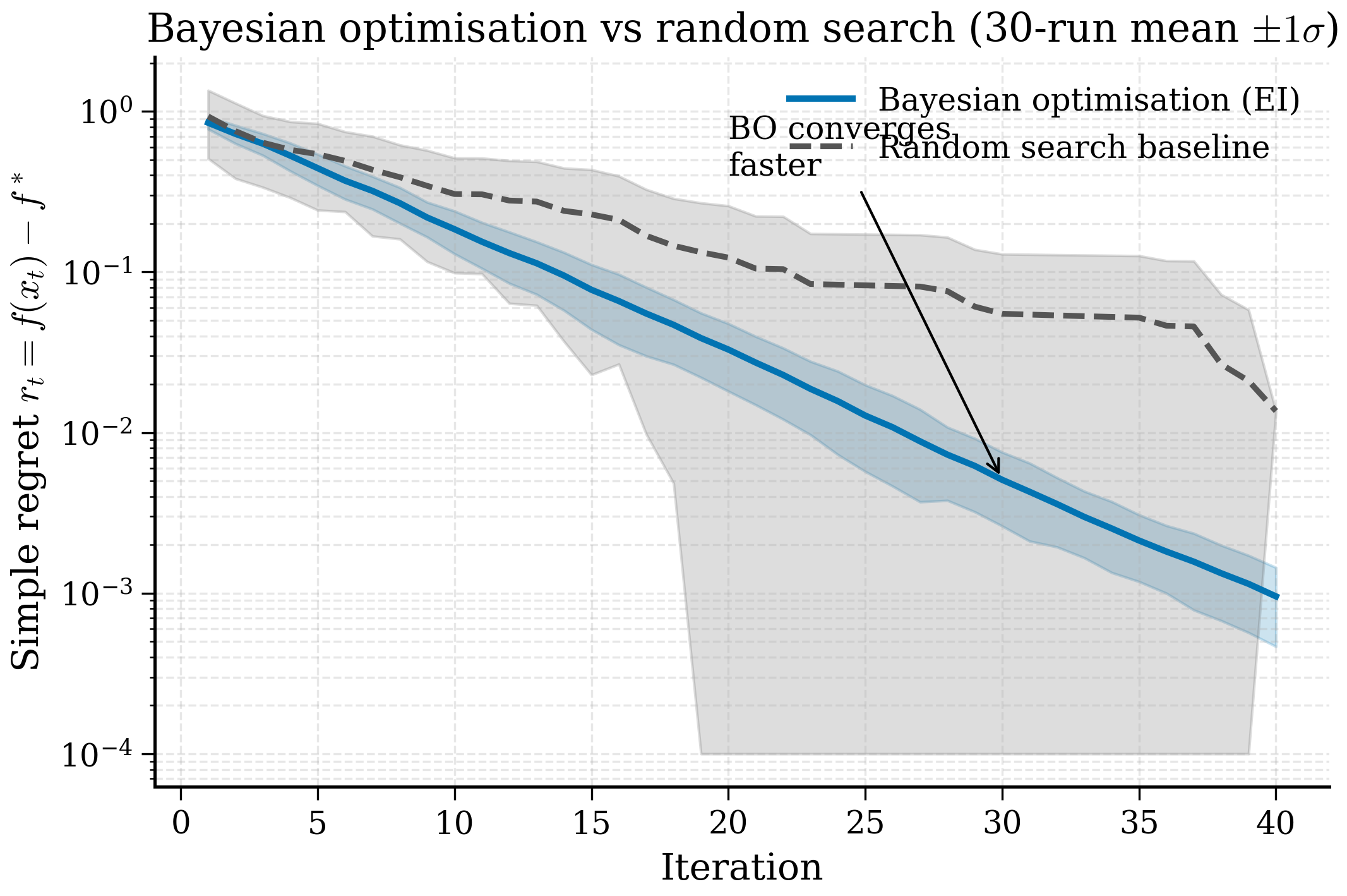
Running this script on a laptop takes about 10 minutes (50 iterations × 30 seeds × ~1 s per GP fit). The resulting plot (Figure 11.4.1) shows BO reaching simple regret $\sim 0.05$ in about 15 iterations, while random search needs $\sim 100$ iterations to reach the same regret — a roughly $7\times$ advantage. Note the log y-axis: the gap is even more pronounced than it appears at first glance.

The same script with the synthetic objective replaced by a DFT-backed oracle becomes a real materials BO campaign. Substitute synthetic_objective(X) with a function that runs DFT (using ASE/VASP/Quantum ESPRESSO) on the structure encoded by X, and the loop drives a real screening campaign. The only practical wrinkle is caching: store DFT results in a database so re-running the script does not duplicate work.

11.4.7 Where this leaves us¶

Chapter 11 has built, from first principles, the tools that turn a fast surrogate (Chapter 10) into a budget-aware discovery loop. The mathematical content was the Gaussian process and its acquisition functions; the materials content was featurisation and oracle selection; the practical content was BoTorch and the autonomous-lab exemplar.

Chapter 12 takes the next step: foundation models for materials — universally pre-trained networks whose representations make the featurisation problem nearly trivial and whose fine-tuning makes the surrogate fitting nearly automatic. In the chapter-12 framing, the BO loop becomes one ingredient in a much larger machine that ingests any materials question and returns the next experiment to run. The conceptual content of Chapter 11 — the exploration-exploitation trade-off and the acquisition functions that formalise it — persists unchanged into that larger machine. It is the part of materials ML that no amount of foundation-model scale displaces.

Section summary¶

Featurise candidates with Magpie (cheap, composition-only), structural descriptors (SOAP/ACSF for crystals), or GNN embeddings (best for structure-dependent properties).
Oracle choices: DFT (slow, accurate), MLIP (fast, approximate); multi-fidelity BO couples them via co-kriging.
Closed-loop autonomous experimentation (A-Lab, MIT-IBM Watson) is the production case study; key lessons are tight cycles, failure logging, and uncertainty calibration.
Constraints and multi-objective extensions are well-supported in BoTorch via ConstrainedExpectedImprovement and qExpectedHypervolumeImprovement.

Remark 11.4.5 — selecting an initial design

The first 5–20 queries in any BO campaign are not chosen by an acquisition function (the GP has no data to fit). They are chosen by a space-filling design: random sampling, Latin hypercube sampling (LHS), or Sobol sequences. Of the three, LHS is the most commonly recommended: it guarantees that the marginal distribution of each input dimension is uniform, avoiding random sampling's occasional clusters and gaps. Sobol sequences offer slightly better space-filling for low dimensions but become less reliable above 10D. Sample size: 5 + $d$ where $d$ is input dimension is a common rule of thumb; for the perovskite example with $d \sim 30$ (Magpie features), the initial 3 was deliberately small to illustrate the loop, and a real campaign would use $\sim 30$.

Section summary (already listed above)¶

Regret curve interpretation

A simple regret curve plots best-found value as a function of iteration. A cumulative regret curve plots total suboptimality. For materials discovery the right metric is usually simple regret — you care only about the best material found, not the average. The example regret curve in Fig 11.4.1 shows BO reaching low simple regret in $\sim 15$ iterations where random search needs $\sim 100$; this $\sim 7\times$ advantage is typical of well-tuned BO on smooth objectives, and grows with dimensionality.