11.2 Gaussian Processes

Figure 11.2.1. (Left) Samples from a Gaussian-process prior with an RBF kernel — smooth functions whose pointwise marginals lie within the grey \(\pm 2\sigma\) band. (Right) Conditioning on three noiseless observations collapses the posterior to a narrow band around the data and inflates uncertainty between them.

The probabilistic surrogate that has dominated Bayesian optimisation for twenty years is the Gaussian process (GP). It is a model of the unknown function that, given any finite set of input points, returns a multivariate Gaussian distribution over the function values at those points. The Gaussian distribution comes equipped with a mean and a covariance, which translate directly into a predicted value and an uncertainty — exactly the two ingredients §11.1 argued we need.

This section develops GPs from the definition, derives the predictive posterior step by step, discusses hyperparameter selection, and ends with a NumPy implementation of GP regression on a toy 1D problem. The maths is occasionally heavy; the payoff is that the implementation in §11.2.6 is fewer than eighty lines and trivially adaptable to any materials regression problem.

Why this is the hardest section in Chapter 11

Gaussian processes require Gaussian linear algebra to be at one's fingertips. Two facts about multivariate Gaussians do all the work: (i) any marginal of a joint Gaussian is Gaussian, and (ii) any conditional of a joint Gaussian is Gaussian, with explicit formulas. Once these are second nature, GP regression is a one-line application; until then, the formulae look impenetrable. We rehearse the linear algebra carefully in §11.2.4 before deploying it.

Key Idea (Box 11.2.A)

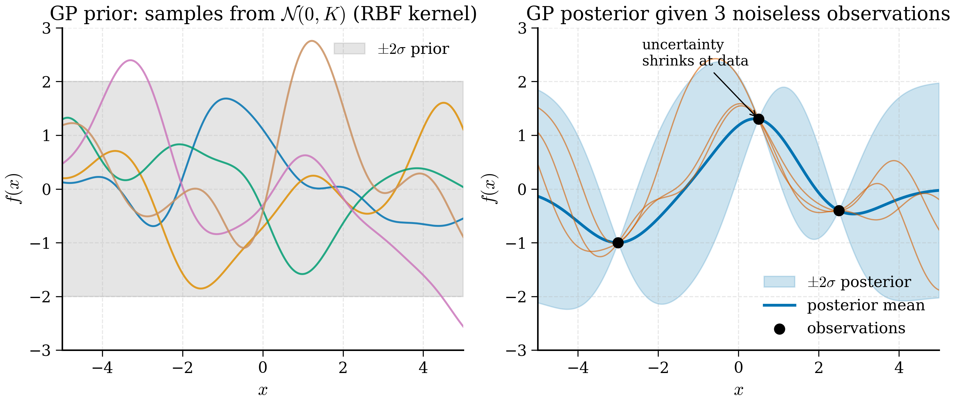
A Gaussian process is a probability distribution over functions: any finite collection of function values, at any inputs, is jointly Gaussian. Specified by a mean function and a kernel, a GP delivers — for every test input — a posterior mean and a posterior variance, exactly the two ingredients required for decision-making under uncertainty.

11.2.1 Definition

A Gaussian process on input space \(\mathcal{X} \subset \mathbb{R}^d\) is a collection of random variables \(\{f(\mathbf{x})\}_{\mathbf{x} \in \mathcal{X}}\) indexed by inputs \(\mathbf{x}\), such that for any finite collection \(\{\mathbf{x}_1, \ldots, \mathbf{x}_n\} \subset \mathcal{X}\), the joint distribution of \([f(\mathbf{x}_1), \ldots, f(\mathbf{x}_n)]^T\) is multivariate Gaussian.

A GP is fully specified by a mean function and a covariance function (also called a kernel): $$ m(\mathbf{x}) = \mathbb{E}[f(\mathbf{x})], \qquad k(\mathbf{x}, \mathbf{x}') = \mathbb{E}\big[(f(\mathbf{x}) - m(\mathbf{x}))(f(\mathbf{x}') - m(\mathbf{x}'))\big]. $$ We write \(f \sim \mathcal{GP}(m, k)\).

For any finite set of inputs \(X = [\mathbf{x}_1, \ldots, \mathbf{x}_n]^T\), the joint distribution of \(\mathbf{f} = [f(\mathbf{x}_1), \ldots, f(\mathbf{x}_n)]^T\) is $$ \mathbf{f} \sim \mathcal{N}(\mathbf{m}, K), $$ where \(\mathbf{m}_i = m(\mathbf{x}_i)\) and \(K_{ij} = k(\mathbf{x}_i, \mathbf{x}_j)\).

In essentially every practical application the mean function is set to zero — without loss of generality, since the data can be centred — and the kernel does all the work.

Intuition: a GP as an infinite-dimensional Gaussian

A multivariate Gaussian over \(\mathbb{R}^n\) is parametrised by an \(n\)-dimensional mean and an \(n \times n\) covariance. A GP is the limiting case as \(n \to \infty\): instead of indexing by integer \(i = 1, \ldots, n\), we index by a continuous input \(\mathbf{x}\). The covariance becomes a kernel function \(k(\mathbf{x}, \mathbf{x}')\). Any finite sample from the GP — at inputs \(\mathbf{x}_1, \ldots, \mathbf{x}_n\) — recovers a finite- dimensional Gaussian with mean and covariance computed by evaluating \(m\) and \(k\) pointwise.

This is the formal definition of a stochastic process: a probability distribution over functions. The GP is the most tractable nontrivial example because the marginals are all Gaussian and Gaussians stay Gaussian under conditioning.

Rigorous statement: Kolmogorov consistency

For a collection of finite-dimensional distributions \(\{p(\mathbf{f}_S) : S \subset \mathcal{X} \text{ finite}\}\) to define a single stochastic process, they must satisfy two consistency conditions: (i) exchangeability — the distribution of \(\mathbf{f}_S\) is invariant under reordering the elements of \(S\); (ii) marginal consistency — for \(S \subset T\), the marginal of \(p(\mathbf{f}_T)\) over the extra elements equals \(p(\mathbf{f}_S)\). The Kolmogorov extension theorem (1933) guarantees that any consistent family of finite-dimensional distributions extends to a stochastic process. For GPs, consistency is automatic: marginals of joint Gaussians are Gaussians with the right submatrices of the covariance.

11.2.2 Kernels: the workhorse, RBF

The kernel encodes the user's prior beliefs about the function: smoothness, length scale, output magnitude, periodicity. The most common kernel by a wide margin is the radial basis function (RBF), also called the squared exponential: $$ k_{\mathrm{RBF}}(\mathbf{x}, \mathbf{x}') = \sigma_f^2 \exp!\left(-\frac{|\mathbf{x} - \mathbf{x}'|^2}{2 \ell^2}\right). $$ Two hyperparameters: the output scale \(\sigma_f\) controlling the overall magnitude of function values, and the length scale \(\ell\) controlling how rapidly the function varies. Functions drawn from a GP with this kernel are infinitely differentiable (which is sometimes too smooth for real data; the Matérn family is the standard alternative when functions look rougher).

Properties of a valid kernel:

• Symmetric. \(k(\mathbf{x}, \mathbf{x}') = k(\mathbf{x}', \mathbf{x})\).
• Positive semi-definite. For any finite set of inputs, the matrix \(K\) with entries \(K_{ij} = k(\mathbf{x}_i, \mathbf{x}_j)\) must be positive semi-definite. This guarantees a valid covariance matrix.

The RBF satisfies both. Other useful kernels include:

• Matérn-5/2: \(k = \sigma_f^2 (1 + \sqrt{5} r/\ell + 5 r^2/(3\ell^2)) \exp(-\sqrt{5} r/\ell)\) where \(r = \|\mathbf{x} - \mathbf{x}'\|\). Functions are twice differentiable but not infinitely. Often a better default than RBF for real problems.
• Linear: \(k(\mathbf{x}, \mathbf{x}') = \sigma_f^2 \mathbf{x}^T \mathbf{x}'\). Encodes a linear prior.
• Periodic: \(k(\mathbf{x}, \mathbf{x}') = \sigma_f^2 \exp(-2 \sin^2(\pi |x - x'|/p)/\ell^2)\).

Kernels can be added and multiplied to produce richer priors. For most of this chapter, RBF or Matérn-5/2 with a single length scale will do.

When to use which kernel

A practical guide.

RBF (squared exponential): smooth, infinitely differentiable functions. Default choice when the underlying physics is smooth (formation energies, band gaps as functions of composition). Tends to be over-confident in extrapolation because of its rapid decay.

Matérn-3/2: functions are once differentiable. Use when the underlying signal looks noisy or rough; preferred for many engineering applications. Less smooth than RBF but more honest about uncertainty.

Matérn-5/2: twice differentiable. The sweet spot between RBF's over-smoothness and Matérn-3/2's roughness. BoTorch's default.

Linear: prior is a linear function. Use when the relationship is known to be linear (e.g., interpolating between two end-members in a binary alloy).

Periodic: function repeats with period \(p\). Use when there is explicit periodicity (a property as a function of angle, e.g.).

Sum of kernels \(k_1 + k_2\): prior is sum of two functions, one drawn from \(k_1\) and one from \(k_2\). Useful for trend + residual decompositions.

Product of kernels \(k_1 \times k_2\): more restrictive prior; used for ARD (automatic relevance determination) by combining per-dimension Matérn kernels with different length scales.

Tanimoto / chemical-fingerprint kernels: input is a binary chemical fingerprint; kernel is Tanimoto similarity. Use for molecule property prediction where the natural space is fingerprint Hamming-similar.

Numerical exercise: kernel sensitivity

With three training points \(x_1 = 0, x_2 = 1, x_3 = 2\) and \(y = (0, 1, 0)\), plot the GP posterior under three kernels: RBF with \(\ell = 0.5\), RBF with \(\ell = 2.0\), and Matérn-3/2 with \(\ell = 0.5\). The RBF with short length scale interpolates with sharp peaks; the RBF with long length scale washes out the structure; the Matérn-3/2 produces a less rounded interpolation, with visible kinks at the data points. The "right" answer depends on what you believe about the underlying function — a judgement that is the prior in Bayesian terminology.

11.2.2a Kernels as inner products: the kernel trick

A complementary view of a kernel is as an inner product in a (possibly infinite-dimensional) feature space. For the RBF kernel, there exists a feature map \(\phi: \mathbb{R}^d \to \mathcal{H}\) into a Hilbert space such that \(k(\mathbf{x}, \mathbf{x}') = \langle \phi(\mathbf{x}), \phi(\mathbf{x}') \rangle_\mathcal{H}\). The feature map is infinite-dimensional and not explicitly computable, but the kernel evaluates the inner product without it — this is the kernel trick.

The consequence is that GP regression is equivalent to linear regression in the feature space \(\mathcal{H}\). The posterior mean \(\mu(\mathbf{x}_*) = \mathbf{k}_*^T (K + \sigma_n^2 I)^{-1} \mathbf{y}\) is the prediction of an infinite-dimensional ridge regression evaluated through the kernel. This perspective makes some properties intuitive: smoothness of the RBF kernel corresponds to using a feature space dominated by low-frequency components, and a GP is just kernel ridge regression with a probabilistic interpretation laid on top.

11.2.3 The regression problem

We are given \(n\) observations \(\mathcal{D} = \{(\mathbf{x}_i, y_i)\}_{i=1}^{n}\) where \(y_i = f(\mathbf{x}_i) + \varepsilon_i\) and \(\varepsilon_i \sim \mathcal{N}(0, \sigma_n^2)\) is i.i.d. observation noise. We assume a GP prior \(f \sim \mathcal{GP}(0, k)\) over the underlying function and wish to predict the function value \(f_* = f(\mathbf{x}_*)\) at a new test input \(\mathbf{x}_*\).

The training-data values \(\mathbf{y} = [y_1, \ldots, y_n]^T\) and the test function value \(f_*\) are jointly Gaussian under the GP prior: $$ \begin{bmatrix} \mathbf{y} \ f_* \end{bmatrix} \sim \mathcal{N}!\left( \mathbf{0}, \begin{bmatrix} K + \sigma_n^2 I & \mathbf{k}* \ \mathbf{k}^T & k_{*} \end{bmatrix} \right), $$ where:

• \(K \in \mathbb{R}^{n \times n}\) has entries \(K_{ij} = k(\mathbf{x}_i, \mathbf{x}_j)\),
• \(\mathbf{k}_* \in \mathbb{R}^{n}\) has entries \(k_{*,i} = k(\mathbf{x}_*, \mathbf{x}_i)\),
• \(k_{**} = k(\mathbf{x}_*, \mathbf{x}_*) \in \mathbb{R}\),
• \(\sigma_n^2 I\) accounts for the noise in \(\mathbf{y}\) but not in \(f_*\) (we want to predict the latent function, not noisy observations).

11.2.4 Conditioning: the predictive posterior

The predictive distribution \(p(f_* \mid \mathbf{y})\) is the conditional of \(f_*\) given \(\mathbf{y}\). For a multivariate Gaussian, conditioning is a closed-form operation. Let us derive it carefully.

Standard result: if $$ \begin{bmatrix} \mathbf{a} \ \mathbf{b} \end{bmatrix} \sim \mathcal{N}!\left( \begin{bmatrix} \boldsymbol{\mu}a \ \boldsymbol{\mu}_b \end{bmatrix}, \begin{bmatrix} \Sigma \ \Sigma_{ba} & \Sigma_{bb} \end{bmatrix} \right), $$ then $$ \mathbf{a} \mid \mathbf{b} \sim \mathcal{N}!\left( \boldsymbol{\mu}} & \Sigma_{aba + \Sigma} \Sigma_{bb}^{-1} (\mathbf{b} - \boldsymbol{\mub),\; \Sigma \right). $$ This is the Gaussian conditioning identity; it follows from completing the square in the joint density.} - \Sigma_{ab} \Sigma_{bb}^{-1} \Sigma_{ba

Derivation: Gaussian conditioning via Schur complement

We derive the conditional density step by step. Start from the joint density $$ p(\mathbf{a}, \mathbf{b}) \propto \exp!\left(-\tfrac{1}{2} \begin{pmatrix}\mathbf{a} \ \mathbf{b}\end{pmatrix}^T \begin{pmatrix}\Sigma_{aa} & \Sigma_{ab} \ \Sigma_{ba} & \Sigma_{bb}\end{pmatrix}^{-1} \begin{pmatrix}\mathbf{a} \ \mathbf{b}\end{pmatrix} \right), $$ with means set to zero for clarity. Block-invert the covariance using the Schur complement of \(\Sigma_{bb}\), \(S = \Sigma_{aa} - \Sigma_{ab} \Sigma_{bb}^{-1} \Sigma_{ba}\): $$ \begin{pmatrix}\Sigma_{aa} & \Sigma_{ab} \ \Sigma_{ba} & \Sigma_{bb}\end{pmatrix}^{-1} = \begin{pmatrix} S^{-1} & -S^{-1} \Sigma_{ab} \Sigma_{bb}^{-1} \ -\Sigma_{bb}^{-1} \Sigma_{ba} S^{-1} & \Sigma_{bb}^{-1} + \Sigma_{bb}^{-1} \Sigma_{ba} S^{-1} \Sigma_{ab} \Sigma_{bb}^{-1} \end{pmatrix}. $$ Expand the quadratic form in the exponent. The terms involving \(\mathbf{a}\) are $$ -\tfrac{1}{2} \mathbf{a}^T S^{-1} \mathbf{a} + \mathbf{a}^T S^{-1} \Sigma_{ab} \Sigma_{bb}^{-1} \mathbf{b} - \tfrac{1}{2} \mathbf{b}^T \Sigma_{bb}^{-1} \Sigma_{ba} S^{-1} \Sigma_{ab} \Sigma_{bb}^{-1} \mathbf{b} + (\text{terms in } \mathbf{b}^T \Sigma_{bb}^{-1} \mathbf{b}). $$ Complete the square in \(\mathbf{a}\). Let \(\boldsymbol{\mu}_{a|b} = \Sigma_{ab} \Sigma_{bb}^{-1} \mathbf{b}\). Then the \(\mathbf{a}\)-dependent terms become \(-\tfrac{1}{2} (\mathbf{a} - \boldsymbol{\mu}_{a|b})^T S^{-1} (\mathbf{a} - \boldsymbol{\mu}_{a|b}) + (\text{constants in } \mathbf{a})\). Reading off: \(\mathbf{a} | \mathbf{b}\) is Gaussian with mean \(\boldsymbol{\mu}_{a|b} = \Sigma_{ab} \Sigma_{bb}^{-1} \mathbf{b}\) and covariance \(S = \Sigma_{aa} - \Sigma_{ab} \Sigma_{bb}^{-1} \Sigma_{ba}\). Adding back the means (we set them to zero) gives the general formula stated above. \(\square\)

The Schur complement \(S\) is the posterior covariance: it equals the prior covariance \(\Sigma_{aa}\) minus a correction that measures how much \(\mathbf{b}\) constrains \(\mathbf{a}\). The correction is positive semidefinite, so observing \(\mathbf{b}\) can only reduce uncertainty.

Theorem 11.2.1 (GP regression predictive distribution)

Let \(f \sim \mathcal{GP}(0, k)\) and let \(\mathcal{D} = \{(\mathbf{x}_i, y_i)\}_{i=1}^n\) be observations with i.i.d. Gaussian noise of variance \(\sigma_n^2\). Then for any test input \(\mathbf{x}_*\) the posterior \(p(f(\mathbf{x}_*) | \mathcal{D})\) is Gaussian with mean and variance given by equations (11.1) and (11.2). Proof. Specialisation of the Gaussian conditioning identity to the joint distribution given in §11.2.3. \(\square\)

Apply it with \(\mathbf{a} = f_*\) and \(\mathbf{b} = \mathbf{y}\), mean zero, \(\Sigma_{aa} = k_{**}\), \(\Sigma_{ab} = \mathbf{k}_*^T\), \(\Sigma_{bb} = K + \sigma_n^2 I\). We obtain $$ \boxed{ \mu(\mathbf{x}) = \mathbf{k}_^T (K + \sigma_n^2 I)^{-1} \mathbf{y}, } \tag{11.1} $$ $$ \boxed{ \sigma^2(\mathbf{x}) = k_{**} - \mathbf{k}_^T (K + \sigma_n^2 I)^{-1} \mathbf{k}_. } \tag{11.2} $$ These are *the GP regression formulae. Three observations.

First, the predictive mean is a linear combination of the training observations \(\mathbf{y}\), with weights \(\boldsymbol{\alpha} = (K + \sigma_n^2 I)^{-1} \mathbf{y}\) that do not depend on \(\mathbf{x}_*\). Computing \(\boldsymbol{\alpha}\) once during training, the mean prediction at a new point is just \(\mathbf{k}_*^T \boldsymbol{\alpha}\) — an \(O(n)\) inner product.

Second, the predictive variance does not depend on the observed values \(\mathbf{y}\) — only on where we have observed and where we are predicting. The GP cannot become "more confident" by seeing values that happen to be consistent with each other; its uncertainty depends only on the geometry of the data. (This is a feature of the GP prior, not a universal property of probabilistic models.)

Third, the cost of GP regression is dominated by the inversion of the \(n \times n\) matrix \(K + \sigma_n^2 I\), which is \(O(n^3)\) in time and \(O(n^2)\) in memory. This scaling limits GPs to roughly \(n \lesssim 10^4\) training points without approximations. For BO, \(n\) rarely exceeds a few hundred — the whole point is that each observation is expensive — so this is rarely a bottleneck.

In practice we never invert \(K + \sigma_n^2 I\) explicitly. Instead we Cholesky-factor it: \(K + \sigma_n^2 I = L L^T\) where \(L\) is lower triangular. Then \(\boldsymbol{\alpha}\) is solved as \(L^T \boldsymbol{\alpha} = L^{-1} \mathbf{y}\) in two triangular solves. The Cholesky route is more numerically stable than direct inversion and is what every production GP library uses.

Numerical stability: jitter

Even with Cholesky factorisation, the matrix \(K + \sigma_n^2 I\) can be ill-conditioned. Two training points very close in input space produce near-duplicate rows in \(K\) (entries close to \(\sigma_f^2\)), which inflates the condition number. Production code adds a small jitter \(\epsilon I\) with \(\epsilon = 10^{-6}\) or so to the diagonal, raising the noise floor enough to make Cholesky succeed without measurably changing the posterior. If jitter at \(10^{-3}\) is needed to make Cholesky succeed, your data has near-duplicate points and you should deduplicate before fitting.

Numerical example: a \(3 \times 3\) kernel matrix

With training inputs \(x_1 = 0, x_2 = 1, x_3 = 3\), RBF kernel (\(\sigma_f = 1, \ell = 1\)), and noise \(\sigma_n = 0.1\): $$ K = \begin{pmatrix} 1 & e^{-½} & e^{-9/2} \ e^{-½} & 1 & e^{-2} \ e^{-9/2} & e^{-2} & 1 \end{pmatrix} \approx \begin{pmatrix} 1 & 0.607 & 0.011 \ 0.607 & 1 & 0.135 \ 0.011 & 0.135 & 1 \end{pmatrix}. $$ Adding \(\sigma_n^2 I = 0.01 I\) gives a well-conditioned matrix with smallest eigenvalue around 0.4 and largest around 1.7. With targets \(\mathbf{y} = (0, 1, -0.5)\), we compute \(\boldsymbol{\alpha} = (K + 0.01 I)^{-1} \mathbf{y}\), which works out to approximately \((-0.62, 1.05, -0.61)\). The posterior mean at a test point \(x_* = 2\) is \(\mathbf{k}_*^T \boldsymbol{\alpha}\) where \(\mathbf{k}_* = (e^{-2}, e^{-1/2}, e^{-1/2}) \approx (0.135, 0.607, 0.607)\), giving \(\mu(2) \approx 0.55\). The posterior variance is \(k_{**} - \mathbf{k}_*^T (K + 0.01 I)^{-1} \mathbf{k}_* \approx 1 - 0.62 = 0.38\), so \(\sigma(2) \approx 0.62\). The prediction is "between the values at \(x=1\) and \(x=3\) but with substantial uncertainty" — exactly what we would expect of a GP interpolating from sparse data.

Pause and recall

Before reading on, try to answer these from memory:

1. What two functions fully specify a Gaussian process, and what role does the kernel play in encoding prior beliefs?
2. Write down (in words) the GP predictive mean and variance — why does the predictive variance not depend on the observed values \(\mathbf{y}\)?
3. Why is the GP posterior computed via a Cholesky factorisation rather than by explicitly inverting \(K + \sigma_n^2 I\)?

If any of these is shaky, re-read the preceding section before continuing.

11.2.5 Hyperparameter learning by marginal likelihood

The kernel has hyperparameters \(\boldsymbol{\theta} = (\sigma_f, \ell, \sigma_n)\). How do we choose them?

The Bayesian answer is to integrate them out under a prior. The practical answer is maximum marginal likelihood: choose \(\boldsymbol{\theta}\) to maximise $$ p(\mathbf{y} \mid X, \boldsymbol{\theta}) = \mathcal{N}(\mathbf{y}; \mathbf{0}, K_{\boldsymbol{\theta}} + \sigma_n^2 I). $$ The log marginal likelihood is $$ \log p(\mathbf{y} \mid X, \boldsymbol{\theta}) = -\tfrac{1}{2} \mathbf{y}^T (K_{\boldsymbol{\theta}} + \sigma_n^2 I)^{-1} \mathbf{y} - \tfrac{1}{2} \log |K_{\boldsymbol{\theta}} + \sigma_n^2 I| - \tfrac{n}{2} \log 2\pi. \tag{11.3} $$ The three terms have natural interpretations:

• The first term, the data fit, rewards small residuals after whitening by the inverse covariance.
• The second term, the model complexity penalty, grows with the determinant of the covariance; it penalises overly flexible kernels.
• The third term is a constant.

The complexity penalty is automatic Occam's razor: as we make the length scale shorter (more flexible kernel), the data fit improves but the determinant grows and the penalty rises. The optimum balances the two.

We typically optimise \(\log p\) by gradient ascent. The gradient with respect to a hyperparameter \(\theta_j\) is $$ \frac{\partial \log p}{\partial \theta_j} = \tfrac{1}{2} \mathbf{y}^T \tilde K^{-1} \frac{\partial \tilde K}{\partial \theta_j} \tilde K^{-1} \mathbf{y} - \tfrac{1}{2} \mathrm{tr}!\left( \tilde K^{-1} \frac{\partial \tilde K}{\partial \theta_j} \right), $$ where \(\tilde K = K_{\boldsymbol{\theta}} + \sigma_n^2 I\). This is the formula a GP library evaluates at every optimisation step.

The log marginal likelihood is in general non-convex in \(\boldsymbol{\theta}\) — multiple local maxima correspond to different qualitative interpretations of the same data. Restart from several initialisations and check that the answer is consistent.

Derivation: the gradient formula

Write \(\tilde K = K + \sigma_n^2 I\). We need \(\partial / \partial \theta_j\) of \(\log p = -\tfrac{1}{2} \mathbf{y}^T \tilde K^{-1} \mathbf{y} - \tfrac{1}{2} \log |\tilde K| + \text{const}\).

The first term: using the identity \(\partial \tilde K^{-1} / \partial \theta_j = -\tilde K^{-1} (\partial \tilde K / \partial \theta_j) \tilde K^{-1}\), we get \(-\tfrac{1}{2} \partial/\partial\theta_j (\mathbf{y}^T \tilde K^{-1} \mathbf{y}) = \tfrac{1}{2} \mathbf{y}^T \tilde K^{-1} (\partial \tilde K / \partial \theta_j) \tilde K^{-1} \mathbf{y}\).

The second term: using \(\partial \log|\tilde K| / \partial \theta_j = \mathrm{tr}(\tilde K^{-1} \partial \tilde K / \partial \theta_j)\) (Jacobi's formula), \(-\tfrac{1}{2} \partial \log|\tilde K| / \partial \theta_j = -\tfrac{1}{2} \mathrm{tr}(\tilde K^{-1} \partial \tilde K / \partial \theta_j)\).

Combining yields equation given in the main text. The first term is the data-driven push (in the direction that improves fit); the second is the complexity-penalty pull (towards simpler models). At the optimum, the two cancel.

Two local minima from the same data

A famous toy: ten data points roughly on a sine wave with noise. The log marginal likelihood has two prominent local maxima. The first sets \(\ell \approx 1\), \(\sigma_n \approx 0.1\) — interpreting the data as smoothly-varying with small noise. The second sets \(\ell \approx 0.05\), \(\sigma_n \approx 0.5\) — interpreting the data as wildly-varying with large noise (a "white-noise" explanation). Both fit the data equally well; they differ in what they predict for unseen inputs. Running optimisation from several initialisations reveals both, and the user must choose based on prior knowledge.

11.2.6 NumPy implementation

We now implement everything from scratch. The code reproduces a textbook 1D regression example: noisy observations of a sine wave with six training points.

"""Minimal Gaussian process regression in pure NumPy."""

from __future__ import annotations

import numpy as np
from numpy.typing import NDArray
from scipy.linalg import cho_factor, cho_solve
from scipy.optimize import minimize


# ---------------------------------------------------------------------------
# 1. RBF kernel
# ---------------------------------------------------------------------------

def rbf_kernel(
    x1: NDArray[np.float64],
    x2: NDArray[np.float64],
    sigma_f: float,
    length_scale: float,
) -> NDArray[np.float64]:
    """Evaluate the RBF kernel between two sets of inputs.

    x1: shape (n1, d). x2: shape (n2, d). Returns (n1, n2).
    """
    sq = np.sum(x1 ** 2, axis=1, keepdims=True) \
       + np.sum(x2 ** 2, axis=1) \
       - 2.0 * x1 @ x2.T
    sq = np.maximum(sq, 0.0)  # numerical safety
    return sigma_f ** 2 * np.exp(-0.5 * sq / length_scale ** 2)


# ---------------------------------------------------------------------------
# 2. GP regression
# ---------------------------------------------------------------------------

class GP:
    """Gaussian process regression with RBF kernel and Gaussian noise."""

    def __init__(
        self,
        sigma_f: float = 1.0,
        length_scale: float = 1.0,
        sigma_n: float = 0.1,
    ) -> None:
        self.sigma_f = sigma_f
        self.length_scale = length_scale
        self.sigma_n = sigma_n
        self.X: NDArray[np.float64] | None = None
        self.y: NDArray[np.float64] | None = None
        self.alpha: NDArray[np.float64] | None = None
        self.L: NDArray[np.float64] | None = None

    def fit(
        self, X: NDArray[np.float64], y: NDArray[np.float64]
    ) -> None:
        """Cache training data and precompute Cholesky factor."""
        self.X = np.atleast_2d(X)
        if self.X.shape[0] != y.shape[0]:
            self.X = self.X.T
        self.y = y.astype(np.float64)
        K = rbf_kernel(self.X, self.X, self.sigma_f, self.length_scale)
        K += self.sigma_n ** 2 * np.eye(len(self.X))
        self.L, lower = cho_factor(K, lower=True)
        self.alpha = cho_solve((self.L, lower), self.y)

    def predict(
        self, X_star: NDArray[np.float64]
    ) -> tuple[NDArray[np.float64], NDArray[np.float64]]:
        """Predict posterior mean and variance at X_star."""
        assert self.X is not None and self.alpha is not None
        X_star = np.atleast_2d(X_star)
        if X_star.shape[1] != self.X.shape[1]:
            X_star = X_star.T
        K_star = rbf_kernel(self.X, X_star, self.sigma_f, self.length_scale)
        mu = K_star.T @ self.alpha
        v = cho_solve((self.L, True), K_star)
        K_starstar = rbf_kernel(X_star, X_star, self.sigma_f, self.length_scale)
        sigma2 = np.diag(K_starstar) - np.sum(K_star * v, axis=0)
        sigma2 = np.maximum(sigma2, 1e-12)  # numerical floor
        return mu, sigma2

    def log_marginal_likelihood(
        self,
        params: NDArray[np.float64],
        X: NDArray[np.float64],
        y: NDArray[np.float64],
    ) -> float:
        """Negative log marginal likelihood for minimisation."""
        sigma_f, length_scale, sigma_n = np.exp(params)
        K = rbf_kernel(X, X, sigma_f, length_scale)
        K += sigma_n ** 2 * np.eye(len(X))
        try:
            L, lower = cho_factor(K, lower=True)
        except np.linalg.LinAlgError:
            return 1e10
        alpha = cho_solve((L, lower), y)
        nll = 0.5 * y @ alpha
        nll += np.sum(np.log(np.diag(L)))  # = 0.5 log det K
        nll += 0.5 * len(X) * np.log(2 * np.pi)
        return float(nll)

    def optimise_hyperparameters(
        self,
        X: NDArray[np.float64],
        y: NDArray[np.float64],
        n_restarts: int = 5,
    ) -> None:
        """Optimise (sigma_f, length_scale, sigma_n) by L-BFGS."""
        X = np.atleast_2d(X)
        if X.shape[0] != y.shape[0]:
            X = X.T
        best_nll = np.inf
        best_params = None
        rng = np.random.default_rng(0)
        for _ in range(n_restarts):
            init = rng.normal(0.0, 1.0, size=3)  # log-space init
            res = minimize(
                self.log_marginal_likelihood,
                init,
                args=(X, y),
                method="L-BFGS-B",
            )
            if res.fun < best_nll:
                best_nll = res.fun
                best_params = res.x
        assert best_params is not None
        self.sigma_f, self.length_scale, self.sigma_n = np.exp(best_params)
        self.fit(X, y)

A worked example on a noisy sine:

import matplotlib.pyplot as plt

rng = np.random.default_rng(42)
X_train = np.array([[0.5], [1.0], [2.0], [3.5], [4.0], [5.5]])
y_train = np.sin(X_train.flatten()) + rng.normal(0, 0.1, size=6)

gp = GP()
gp.optimise_hyperparameters(X_train, y_train)
print(f"learned sigma_f       = {gp.sigma_f:.3f}")
print(f"learned length_scale  = {gp.length_scale:.3f}")
print(f"learned sigma_n       = {gp.sigma_n:.3f}")

X_test = np.linspace(0, 7, 200).reshape(-1, 1)
mu, var = gp.predict(X_test)
std = np.sqrt(var)

fig, ax = plt.subplots(figsize=(7, 4))
ax.plot(X_test.flatten(), np.sin(X_test.flatten()), "k--", label="truth")
ax.scatter(X_train.flatten(), y_train, s=40, color="red", label="data")
ax.plot(X_test.flatten(), mu, "b-", label="posterior mean")
ax.fill_between(
    X_test.flatten(),
    mu - 2 * std,
    mu + 2 * std,
    alpha=0.2,
    label="$\\pm 2\\sigma$",
)
ax.legend()
plt.tight_layout()
plt.show()

Typical output: learned length scale near 1.5, learned noise near 0.10 (the truth was 0.1), and a posterior that interpolates the data with narrow uncertainty bands at observed points and wider bands between them. At inputs far from any observation — e.g. \(x > 6\) — the uncertainty band widens to roughly \(\sigma_f\), as the GP reverts to the prior.

Try it interactively

Slide the RBF length-scale \(\ell\) and the noise level \(\sigma_n\) to see how the posterior reshapes. Small \(\ell\) produces a wiggly mean that interpolates every point with confidence collapsing between them; large \(\ell\) over-smooths and ignores genuine structure. The noise slider trades fit (low \(\sigma_n\)) against tolerance to measurement error (high \(\sigma_n\)). The 95% predictive band (\(\pm 2\sigma\)) is shaded.

# widget-config
sliders:
  ell:     {min: 0.1,  max: 3.0, step: 0.05, default: 1.0, label: "Length-scale ℓ"}
  sigma_n: {min: 0.01, max: 1.0, step: 0.01, default: 0.1, label: "Noise σ_n"}

# widget — GP posterior with RBF kernel on a noisy-sine dataset
import numpy as np
import matplotlib.pyplot as plt
from scipy.linalg import cho_factor, cho_solve

ell_val = float(ell)
sn_val = float(sigma_n)
sf = 1.0  # signal amplitude held fixed

rng = np.random.default_rng(42)
X = np.array([0.5, 1.0, 2.0, 3.5, 4.0, 5.5])
y = np.sin(X) + rng.normal(0.0, 0.1, size=X.shape)

def rbf(a, b):
    d2 = (a[:, None] - b[None, :]) ** 2
    return sf ** 2 * np.exp(-0.5 * d2 / ell_val ** 2)

K = rbf(X, X) + sn_val ** 2 * np.eye(len(X))
L, low = cho_factor(K, lower=True)
alpha = cho_solve((L, low), y)

X_star = np.linspace(-0.5, 7.0, 250)
Ks = rbf(X, X_star)
Kss = rbf(X_star, X_star)
mu = Ks.T @ alpha
v = cho_solve((L, low), Ks)
var = np.maximum(np.diag(Kss) - np.sum(Ks * v, axis=0), 1e-12)
std = np.sqrt(var)

# Log marginal likelihood, a useful diagnostic.
nll = 0.5 * y @ alpha + np.sum(np.log(np.diag(L))) + 0.5 * len(X) * np.log(2 * np.pi)
print(f"ℓ = {ell_val:.3f}   σ_n = {sn_val:.3f}")
print(f"log marginal likelihood = {-nll:+.3f}")

fig, ax = plt.subplots(figsize=(6.4, 3.8))
ax.plot(X_star, np.sin(X_star), "k--", lw=1.0, label="truth")
ax.fill_between(X_star, mu - 2 * std, mu + 2 * std,
                color="#5e35b1", alpha=0.18, label="±2σ")
ax.plot(X_star, mu, color="#5e35b1", lw=1.8, label="posterior mean")
ax.scatter(X, y, s=42, color="#c62828", zorder=5, label="data")
ax.set_xlabel("x")
ax.set_ylabel("y")
ax.set_title(f"GP posterior, RBF kernel  (ℓ={ell_val:.2f}, σ_n={sn_val:.2f})")
ax.legend(loc="upper right", fontsize=8)
fig.tight_layout()
plt.show()

11.2.6a A deeper worked example: 1D regression with derivation

To bridge from the code to the equations, walk through the GP calculation on a tiny example with all intermediate quantities.

Let the training data be three points: \(X = ((0,), (1,), (3,))\), \(\mathbf{y} = (0.0, 0.9, -0.4)\). Use an RBF kernel with hyperparameters \(\sigma_f = 1.0\), \(\ell = 1.5\), \(\sigma_n = 0.1\).

Step 1. Compute the \(3 \times 3\) kernel matrix \(K\): \(K_{ij} = \exp(-(x_i - x_j)^2 / (2 \cdot 1.5^2))\). Entries: \(K_{12} = \exp(-1/4.5) \approx 0.801\), \(K_{13} = \exp(-9/4.5) \approx 0.135\), \(K_{23} = \exp(-4/4.5) \approx 0.411\), with ones on the diagonal. Add \(\sigma_n^2 I = 0.01 I\): $$ \tilde K = \begin{pmatrix} 1.01 & 0.801 & 0.135 \ 0.801 & 1.01 & 0.411 \ 0.135 & 0.411 & 1.01 \end{pmatrix}. $$

Step 2. Cholesky factor \(\tilde K = L L^T\): \(L_{11} = \sqrt{1.01} \approx 1.005\), \(L_{21} = 0.801/1.005 \approx 0.797\), \(L_{22} = \sqrt{1.01 - 0.797^2} \approx 0.612\), \(L_{31} = 0.135/1.005 \approx 0.134\), \(L_{32} = (0.411 - 0.134 \cdot 0.797)/0.612 \approx 0.497\), \(L_{33} = \sqrt{1.01 - 0.134^2 - 0.497^2} \approx 0.872\).

Step 3. Solve \(L \mathbf{z} = \mathbf{y}\) by forward substitution: \(z_1 = 0.0/1.005 = 0\), \(z_2 = (0.9 - 0.797 \cdot 0)/0.612 \approx 1.471\), \(z_3 = (-0.4 - 0.134 \cdot 0 - 0.497 \cdot 1.471)/0.872 \approx -1.298\).

Step 4. Solve \(L^T \boldsymbol{\alpha} = \mathbf{z}\) by backward substitution: \(\alpha_3 = -1.298/0.872 \approx -1.488\), \(\alpha_2 = (1.471 - 0.497 \cdot (-1.488))/0.612 \approx 3.612\), \(\alpha_1 = (0 - 0.797 \cdot 3.612 - 0.134 \cdot (-1.488))/1.005 \approx -2.665\).

Step 5. Predict at \(x_* = 2\): \(\mathbf{k}_* = (\exp(-4/4.5), \exp(-1/4.5), \exp(-1/4.5)) \approx (0.411, 0.801, 0.801)\). \(\mu(2) = \mathbf{k}_*^T \boldsymbol{\alpha} \approx 0.411 \cdot (-2.665) + 0.801 \cdot 3.612 + 0.801 \cdot (-1.488) \approx 0.605\).

Predictive variance: \(\sigma^2(2) = 1 - \mathbf{k}_*^T \tilde K^{-1} \mathbf{k}_*\). Computing \(\mathbf{k}_*^T \tilde K^{-1} \mathbf{k}_*\) via the same Cholesky decomposition gives approximately \(0.78\), so \(\sigma(2) \approx \sqrt{0.22} \approx 0.47\).

The interpretation: at \(x = 2\) — halfway between the closest training points at \(x = 1, 3\) — the predicted value is \(0.6\) with one standard deviation about \(\pm 0.47\). The posterior interpolates between the observed values (0.9 at \(x=1\), \(-0.4\) at \(x=3\)) with substantial uncertainty because the points are well-separated relative to the length scale.

11.2.6b Common failure modes

Three failure modes recur in practice.

Length scale collapses to zero. During hyperparameter optimisation, the marginal likelihood maximum drifts to \(\ell \to 0\) (every training point becomes its own cluster) with \(\sigma_n\) explaining the rest. The GP becomes useless: posterior mean at unseen points is zero, posterior variance is \(\sigma_f^2\). Causes: too few training points, or training points that are genuinely scattered with no underlying smooth signal. Fix: bound \(\ell\) from below in the optimiser, or add a prior penalising small \(\ell\).

Length scale explodes to infinity. The opposite: \(\ell \to \infty\) makes \(K\) collapse to the all-ones matrix and the GP becomes a constant predictor. Causes: a target that is nearly constant on the training inputs. Fix: again, prior bounds; or check that the data has non-trivial signal.

Noise level collapses to zero. With \(\sigma_n \to 0\) the GP becomes an exact interpolator; it must pass through every training point. If the data is noisy this is wrong. Fix: prior on \(\sigma_n\), typically log-normal centred at the expected noise level.

The deeper lesson is that GP hyperparameters interact. Length scale, output scale and noise level form a three-way trade-off; a "bad solution" usually involves two of them moving in compensating ways. The marginal likelihood optimisation knows this but does not know what is physically sensible; you do, and should encode it as a prior.

11.2.6c Sparse GPs and scaling

The \(O(n^3)\) scaling restricts vanilla GPs to \(n \lesssim 10^4\). For larger datasets, sparse approximations replace the full kernel matrix with a low-rank approximation built from \(m \ll n\) inducing points \(\mathbf{u}_1, \ldots, \mathbf{u}_m\). The cost drops to \(O(nm^2)\).

The two standard variants are FITC (Snelson and Ghahramani, 2006) and the variational VFE/SVGP (Titsias, 2009; Hensman et al., 2013). VFE is the modern default: it provides a lower bound on the marginal likelihood that can be optimised stochastically over mini-batches, making GPs practical for \(n \sim 10^6\) at the cost of approximation error that depends on \(m\) and on how well the inducing points cover the input space.

For BO, \(n\) is rarely large enough to need sparse GPs. For property regression on the full Materials Project (\(n \sim 10^5\)) sparse GPs are indispensable.

11.2.7 Where we are

We now have a complete, working Gaussian process regressor. It supplies two outputs at every input — a posterior mean \(\mu(\mathbf{x})\) and a posterior variance \(\sigma^2(\mathbf{x})\). Section 11.3 builds acquisition functions that combine these two into a single scalar to optimise, closing the loop on Bayesian optimisation.

Why GPs and not Bayesian neural networks?

A Bayesian neural network places a prior over the weights of a neural network and computes the posterior given the data. In principle this is the right generalisation: more expressive than a GP, equally Bayesian. In practice the posterior over weights is intractable (an exponentially large integral), and the variational approximations introduce their own errors. For \(n \lesssim 10^3\) data points, GPs typically outperform Bayesian neural networks on calibration of uncertainty estimates, which is the only metric that matters for BO. For \(n \gtrsim 10^5\), the situation reverses because GPs become computationally infeasible and the BNN approximations stabilise. The crossover is somewhere around \(n = 10^4\) depending on dimensionality.

For Chapter 11's BO context, \(n\) rarely exceeds a few hundred and the GP wins.

Section summary

• A Gaussian process \(f \sim \mathcal{GP}(m, k)\) is defined by its mean function and kernel; any finite-input marginal is multivariate Gaussian.
• The predictive posterior is given by Theorem 11.2.1; key formulae are (11.1) for \(\mu\) and (11.2) for \(\sigma^2\).
• Hyperparameters \((\sigma_f, \ell, \sigma_n)\) are learned by maximising the log marginal likelihood (11.3); the complexity penalty term implements automatic Occam's razor.
• Standard kernels: RBF (smooth), Matérn-5/2 (default in BoTorch), Matérn-3/2 (rougher), linear (linear prior), periodic. Add/multiply to combine.
• Cost is \(O(n^3)\) for fitting, \(O(n^2)\) for prediction — sparse GPs scale to \(n \gtrsim 10^4\).

A few caveats worth flagging before moving on.

GPs scale as \(O(n^3)\), which limits their applicability to small data. For BO this is rarely a problem; for general regression on thousands of materials it is. Sparse GPs (FITC, VFE), inducing-point approximations and deep kernel learning extend GPs to larger \(n\) at the cost of additional approximation error.

GP predictions extrapolate poorly. The posterior mean reverts to the prior mean (zero, by convention) far from the data; the posterior variance grows to \(\sigma_f^2\). This is the right behaviour by construction — a GP is honest about not knowing what it has not seen — but it limits the utility of GPs for screening campaigns over millions of candidates outside the training distribution.

The choice of kernel determines the answer. RBF and Matérn behave similarly for most problems; specialised kernels matter when the function structure is non-generic (periodic, or with sharp discontinuities). For materials, a Tanimoto kernel on chemical fingerprints, or a string kernel on SMILES, can outperform a generic RBF.

These caveats notwithstanding, the GP is the right starting point for any BO problem with \(n \lesssim 10^4\) observations in a moderate- dimensional input space. The next section turns this surrogate into a decision-making tool by adding acquisition functions on top.

Connecting GP to neural-network surrogates

A natural question: why use a GP at all when CGCNN (Chapter 10) gives faster predictions over the same inputs? The answer is uncertainty. A vanilla CGCNN provides only point predictions; BO needs \((\mu, \sigma)\) per candidate. Three routes deliver this from a neural network:

1. Deep ensembles — train \(M\) networks; mean and std across the ensemble. Calibrated but expensive (\(M\times\) training).
2. MC dropout — apply dropout at inference time; samples give \(\sigma\). Cheap but often miscalibrated.
3. Last-layer Bayesian — replace the final linear layer with a Bayesian linear regression on the network's penultimate features. Cheap and reasonably calibrated.

A GP on the penultimate features of a trained CGCNN combines the expressivity of the neural network with the calibrated uncertainty of a GP. This deep kernel learning construction (Wilson et al., 2016) is the basis of much modern BO for materials, and we will use it in §11.4.

Forward reference

Chapter 11.4 uses the GP machinery developed here with three practical adaptations: (i) inputs are featurised compositions (Magpie features or CGCNN embeddings), (ii) the GP is fitted with BoTorch's GPyTorch backend rather than the NumPy implementation of §11.2.6, and (iii) acquisition functions (§11.3) replace the plain posterior as the decision rule. The mathematical content above carries through unchanged; what changes is the implementation language.

Computational cost of GP fitting in practice

On a 2024 laptop CPU, fitting a vanilla GP with the NumPy implementation of §11.2.6 to 100 training points takes approximately 10 ms (Cholesky factorisation dominates). Hyperparameter optimisation with five L-BFGS restarts adds about 0.5 s. Prediction at 1000 test points is 5 ms (one matrix-vector multiplication).

At 1000 training points, fitting takes 0.5 s and hyperparameter optimisation about 30 s. At 10 000 training points, fitting takes 50 s and hyperparameter optimisation about 30 minutes — the practical limit before sparse approximations are needed.

For BO with \(n \leq 200\) observations, GP fitting is essentially free; the dominant cost is the oracle (DFT, synthesis). This asymmetry is why GPs dominate BO: the cost structure of the problem matches the cost structure of the algorithm.

GPs in higher dimensions: curse and remedies

A 1D GP on a smooth function is essentially perfect with a handful of points. A 10D GP on a smooth function needs exponentially more data because volume in input space scales with dimension. This is the curse of dimensionality and it bites BO sharply: in 20D, even 1000 random points cover the unit hypercube so sparsely that the GP defaults to its prior almost everywhere.

Two remedies. Dimensionality reduction: project inputs to a low-dimensional latent space (PCA, autoencoder, GNN embedding) before GP fitting. Additive kernels: assume the function decomposes as \(f(\mathbf{x}) = \sum_i f_i(x_i)\), fitting one 1D GP per dimension and adding. For composition-driven materials BO, the GNN-embedding route (§11.4) is the standard answer.