4.4 The harmonic oscillator¶

The first four eigenstates of the 1D quantum harmonic oscillator drawn on the parabolic potential well, with energy levels equally spaced by h-bar omega and the ground state sitting at the zero-point energy one half h-bar omega above the potential minimum — Figure 4.4.1. The first four eigenstates of the 1D quantum harmonic oscillator. Energy levels are equally spaced by $\hbar\omega$; the ground state sits at the zero-point energy $\tfrac{1}{2}\hbar\omega$ above the classical minimum.

A comparison of the Morse potential and its harmonic approximation: the two curves share the same curvature at the minimum, but the Morse potential is asymmetric and flattens to a dissociation limit at large bond length while the harmonic parabola rises without bound — Figure 4.4.2. The Morse potential and its harmonic approximation. Both share the same curvature at the minimum, but the Morse potential dissociates at large $r$ and is asymmetric — physically more realistic for molecular bonds. The harmonic approximation is excellent for small displacements only.

If the particle in a box was the simplest non-trivial bound-state problem, the harmonic oscillator is the most useful. Every analytical reflex in quantum mechanics is sharpened on it, every textbook devotes a chapter to it, and — most importantly for materials physics — every potential energy surface looks like a harmonic oscillator near its minimum. The vibrations of a diatomic molecule, the phonons of a crystal, the photons of a quantised electromagnetic field, and the modes of a quantum field are all harmonic oscillators.

This section solves the quantum harmonic oscillator twice. First we present the analytical eigenvalues and eigenfunctions, sketch how they arise (the operator-method derivation is left to the exercises), and meet the zero-point energy. Then we plug the harmonic potential into the finite-difference code of §4.3, recover the spectrum, and finally connect the result to phonons and vibrational spectroscopy in real materials.

4.4.1 Why the harmonic oscillator is universal¶

Consider a one-dimensional system with a smooth potential $V(x)$ that has a local minimum at $x = x_0$. Taylor-expand $V$ around $x_0$:

\[V(x) = V(x_0) + V'(x_0)(x - x_0) + \tfrac12 V''(x_0)(x - x_0)^2 + \tfrac{1}{6}V'''(x_0)(x - x_0)^3 + \cdots \tag{4.4.1}\]

At a minimum, $V'(x_0) = 0$ by definition. Shift the origin to $x_0$ and drop the constant $V(x_0)$ (which only adds a constant to the energy):

\[V(x) \approx \tfrac12 V''(x_0) x^2 + \mathcal O(x^3). \tag{4.4.2}\]

For motion small enough that the cubic and higher terms can be neglected, the system is a harmonic oscillator with spring constant $k = V''(x_0)$. Writing $k = m\omega^2$, the Hamiltonian is

\[\hat{H} = -\frac{\hbar^2}{2m}\frac{d^2}{dx^2} + \tfrac12 m\omega^2 x^2. \tag{4.4.3}\]

This is the canonical form. The angular frequency $\omega$ is the same one a classical particle would oscillate at, $\omega = \sqrt{V''(x_0)/m}$.

The lesson

Whenever you ask a quantum-mechanical question about small deviations from equilibrium, the harmonic oscillator is the right starting point. In Chapter 7 we will compute vibrational frequencies of molecules and phonons of crystals by precisely this procedure: locate equilibrium, compute the Hessian $V''$ (the "force-constant matrix"), diagonalise it to obtain the normal modes — each of which is, by construction, a harmonic oscillator.

Natural units by dimensional analysis¶

Before diving into the eigenvalue problem it is worth asking: what are the natural length, momentum and energy scales of the Hamiltonian (4.4.3)? The parameters available are $\hbar$ (J s), $m$ (kg), and $\omega$ (s$^{-1}$). There is a unique length, momentum and energy formable from these:

\[x_0 \equiv \sqrt{\frac{\hbar}{m\omega}}, \qquad p_0 \equiv \sqrt{\hbar m \omega}, \qquad E_0 \equiv \hbar\omega. \tag{4.4.D1}\]

Why this step? — building scales by dimensional analysis

We need $[x_0] = $ m. From $\hbar$ (units kg m$^2$ s$^{-1}$), $m$ (kg) and $\omega$ (s$^{-1}$), the combination with units of m$^2$ is $\hbar/(m\omega)$; take the square root for a length. Repeat for $p_0$ (units kg m s$^{-1}$) and $E_0$ (units kg m$^2$ s$^{-2}$). The check $x_0 p_0 = \sqrt{(\hbar/m\omega)(\hbar m\omega)} = \hbar$ shows that position and momentum scales saturate the Heisenberg uncertainty product. The HO ground state will indeed be a minimum-uncertainty wavepacket — a sharper version of the result we just saw for the particle in a box.

For an oscillating diatomic molecule with $\omega \sim 10^{14}$ rad/s and $m \sim m_e$, $x_0 \sim 0.3$ Å — the same order as a chemical bond length. For an electron in a magnetic field oscillating at the cyclotron frequency $\omega_c = eB/m$ with $B = 1$ T, $\omega_c \approx 1.8\times 10^{11}$ s$^{-1}$ and $x_0 \approx 26$ nm — the magnetic length. The HO length sets the spatial scale of the wavefunction. Every numerical SHO calculation must put its simulation box at "many $x_0$" or the wavefunction will be clipped at the walls.

4.4.2 The analytical spectrum¶

The eigenvalue problem $\hat{H} \psi = E\psi$ for the Hamiltonian (4.4.3) is the equation

\[-\frac{\hbar^2}{2m} \psi'' + \tfrac12 m\omega^2 x^2 \psi = E\psi. \tag{4.4.4}\]

It is convenient to introduce a dimensionless coordinate. Define the oscillator length

\[\ell \equiv \sqrt{\frac{\hbar}{m\omega}}, \tag{4.4.5}\]

and let $\xi = x/\ell$. The equation becomes

\[-\frac{1}{2}\psi''(\xi) + \frac{1}{2}\xi^2 \psi(\xi) = \frac{E}{\hbar\omega}\psi(\xi). \tag{4.4.6}\]

Writing $\varepsilon \equiv E/(\hbar\omega)$,

\[\psi''(\xi) = (\xi^2 - 2\varepsilon)\psi(\xi). \tag{4.4.7}\]

There are now two paths to the spectrum. The series-solution method (used in nearly every textbook) makes the asymptotic substitution $\psi(\xi) = H(\xi)\, e^{-\xi^2/2}$, derives the Hermite differential equation for $H$, and observes that polynomial solutions exist only when $\varepsilon = n + \tfrac12$ for non-negative integers $n$. The operator-ladder method (due to Dirac) introduces creation and annihilation operators $\hat a^\dagger, \hat a$ satisfying $[\hat a, \hat a^\dagger] = 1$ and shows that $\hat{H} = \hbar\omega(\hat a^\dagger \hat a + \tfrac12)$ has eigenvalues $\hbar\omega(n + \tfrac12)$ for $n = 0, 1, 2, \ldots$

The ladder method in full¶

The operator approach is elegant enough — and useful enough downstream, when we quantise fields and phonons — that we work it through completely here. Introduce the dimensionless position and momentum operators

\[\hat X \equiv \hat x/x_0, \qquad \hat P \equiv \hat p\, x_0/\hbar.\]

These satisfy $[\hat X, \hat P] = i$, by direct substitution into $[\hat x, \hat p] = i\hbar$. The Hamiltonian (4.4.3) becomes

\[\hat H = \frac{\hbar\omega}{2}\left(\hat P^2 + \hat X^2\right).\]

Now define the annihilation and creation operators

\[\boxed{\;\hat a \equiv \frac{1}{\sqrt 2}(\hat X + i\hat P), \qquad \hat a^\dagger \equiv \frac{1}{\sqrt 2}(\hat X - i\hat P).\;} \tag{4.4.L1}\]

Both are non-Hermitian; $\hat a$ and $\hat a^\dagger$ are adjoints of each other. Their commutator is

\[[\hat a, \hat a^\dagger] = \tfrac12[(\hat X + i\hat P), (\hat X - i\hat P)] = \tfrac12(-i[\hat X, \hat P] + i[\hat P, \hat X]) = -i\cdot i = 1.\]

Why this step?

The cross-terms in $[\hat X + i\hat P, \hat X - i\hat P]$ are $-i[\hat X, \hat P] + i[\hat P, \hat X] = -i(i) + i(-i) = 1 + 1 = 2$, divided by 2 gives 1. The non-trivial commutator $[\hat a, \hat a^\dagger] = 1$ is the algebraic statement of canonical quantisation, recast in a basis where the Hamiltonian becomes diagonal.

The Hamiltonian factorises:

\[\hat a^\dagger \hat a = \tfrac12 (\hat X - i\hat P)(\hat X + i\hat P) = \tfrac12(\hat X^2 + \hat P^2 + i[\hat X, \hat P]) = \tfrac12(\hat X^2 + \hat P^2) - \tfrac12,\]

so

\[\hat H = \hbar\omega\,(\hat a^\dagger \hat a + \tfrac12) \equiv \hbar\omega\,(\hat N + \tfrac12), \tag{4.4.L2}\]

where $\hat N \equiv \hat a^\dagger \hat a$ is the number operator.

Now the algebra does the work. If $|\nu\rangle$ is an eigenstate of $\hat N$ with eigenvalue $\nu$, then so are $\hat a|\nu\rangle$ and $\hat a^\dagger|\nu\rangle$, with eigenvalues $\nu - 1$ and $\nu + 1$ respectively:

\[\hat a |0\rangle = 0. \tag{4.4.L3}\]

The full spectrum is $\hat N|n\rangle = n|n\rangle$ for $n = 0, 1, 2, \ldots$, and from (4.4.L2),

\[E_n = \hbar\omega(n + \tfrac12). \quad\checkmark\]

We have recovered (4.4.8) without ever solving the differential equation.

The ground-state wavefunction follows from (4.4.L3) in position representation: $\hat a |0\rangle = \tfrac{1}{\sqrt 2}(\hat X + i\hat P)|0\rangle = 0$ becomes $(\xi + \partial_\xi)\psi_0 = 0$, with solution $\psi_0(\xi) \propto e^{-\xi^2/2}$ — a Gaussian, in agreement with (4.4.9). Excited states are generated by $|n\rangle = (\hat a^\dagger)^n/\sqrt{n!}\;|0\rangle$, which automatically produces the Hermite polynomials.

Why ladder operators matter beyond the SHO

Every quantised harmonic system — phonons in a crystal, photons in a cavity, magnons in a magnet, plasmons in a metal — has the same algebraic structure: a creation operator that adds one quantum and an annihilation operator that removes one. The state with $n$ quanta is $(\hat a^\dagger)^n|0\rangle/\sqrt{n!}$. Quantum field theory is, in a precise sense, just a great many coupled oscillators with this ladder structure. The few pages of algebra you just read are the seed of an enormous tree.

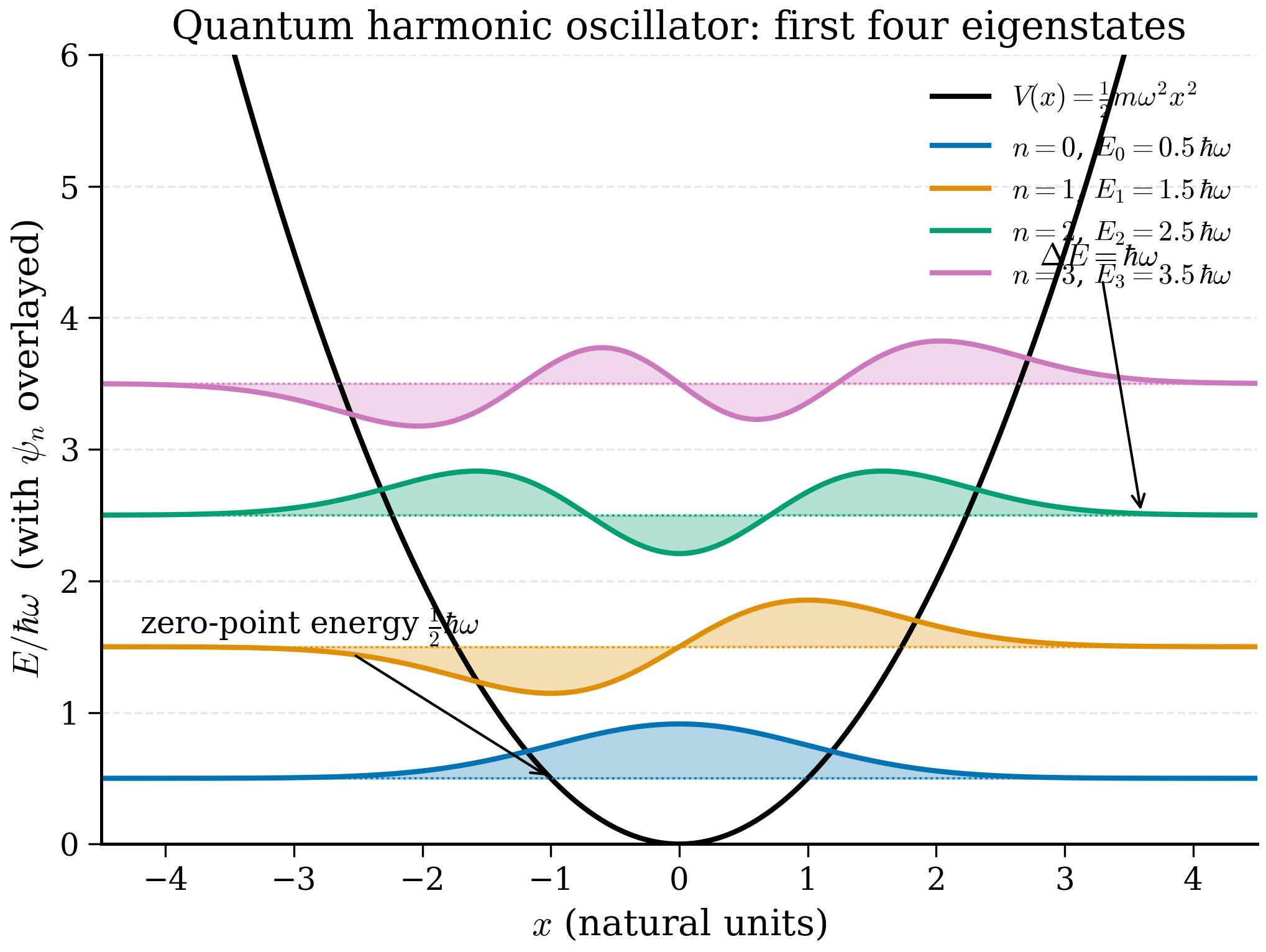
Either way the result is the same: the energy eigenvalues are

\[\boxed{\; E_n = \hbar\omega\left(n + \frac{1}{2}\right), \quad n = 0, 1, 2, \ldots \;} \tag{4.4.8}\]

with corresponding eigenfunctions

\[\psi_n(x) = \frac{1}{\sqrt{2^n n!}}\left(\frac{m\omega}{\pi\hbar}\right)^{1/4} H_n\!\left(\sqrt{\frac{m\omega}{\hbar}}\, x\right) \exp\!\left(-\frac{m\omega x^2}{2\hbar}\right), \tag{4.4.9}\]

where $H_n(\xi)$ are the Hermite polynomials. The first three are

\[H_0(\xi) = 1, \quad H_1(\xi) = 2\xi, \quad H_2(\xi) = 4\xi^2 - 2. \tag{4.4.10}\]

They obey the recursion $H_{n+1}(\xi) = 2\xi H_n(\xi) - 2n H_{n-1}(\xi)$ and the orthogonality $\int_{-\infty}^{\infty} H_m(\xi)H_n(\xi) e^{-\xi^2}d\xi = \sqrt\pi\, 2^n n!\,\delta_{mn}$, which is what makes the prefactor in (4.4.9) the right normalisation. The ground state $\psi_0$ is a pure Gaussian centred on the minimum; the excited states are Gaussians multiplied by polynomials with $n$ real zeros — the standard "$n$ nodes between the classical turning points" pattern.

4.4.3 The zero-point energy¶

The ground-state energy is

\[E_0 = \tfrac12 \hbar\omega. \tag{4.4.11}\]

This is not zero. Unlike a classical oscillator, which can sit motionless at the bottom of its well with $E = 0$, a quantum oscillator has irreducible zero-point motion. There are two complementary ways to see why this must be so.

Uncertainty argument. The Heisenberg uncertainty principle (which follows from the commutator $[\hat x, \hat p] = i\hbar$) says $\Delta x\, \Delta p \geq \hbar/2$. For an oscillator the average energy is $\langle H\rangle = \langle p^2\rangle/2m + \tfrac12 m\omega^2 \langle x^2\rangle = (\Delta p)^2/(2m) + \tfrac12 m\omega^2 (\Delta x)^2$ (using symmetry to set $\langle x\rangle = \langle p\rangle = 0$). Minimising this over $\Delta x$ subject to $\Delta x \cdot \Delta p \geq \hbar/2$ gives $\langle H\rangle_{\min} = \tfrac12\hbar\omega$. Localising the particle costs kinetic energy.

Operator argument. Write $\hat{H} = \hbar\omega(\hat a^\dagger \hat a + \tfrac12)$. Since $\hat a^\dagger \hat a$ is positive semi-definite (it has eigenvalues $0, 1, 2, \ldots$, the "number operator"), the lowest eigenvalue of $\hat{H}$ is $\tfrac12\hbar\omega$, attained on the state with $\hat a |0\rangle = 0$.

The zero-point energy has real physical consequences.

Helium does not solidify at atmospheric pressure even at $T = 0$. The mass is so small and the inter-atomic forces so weak that zero-point motion of the He atoms exceeds the binding-energy minimum, and the system remains liquid. This is the only superfluid in the periodic table.
Lattice constants are temperature-dependent at $T = 0$. Even at absolute zero, atoms vibrate around their equilibrium positions; this zero-point delocalisation slightly expands the lattice, an effect that is now routinely computed for accurate equation-of-state work.
Isotope effects in vibrational spectra: replacing $^1$H with $^2$H (deuterium) halves the zero-point energy of an O–H stretch, shifting absorption lines by 30%. This is the basis of vibrational mode assignment in infrared spectroscopy.
Casimir-style cavity effects in electromagnetism are zero-point energies of photon harmonic oscillators in a confined geometry.

Numerical: zero-point energy of H$_2$

The H$_2$ molecule has a vibrational wavenumber $\tilde\nu \approx 4400$ cm$^{-1}$. Convert to angular frequency: $\omega = 2\pi c \tilde\nu = 2\pi(3\times 10^{10}\,\text{cm/s})(4400\,\text{cm}^{-1}) \approx 8.3\times 10^{14}$ s$^{-1}$. Then $$E_0 = \tfrac12 \hbar\omega = \tfrac12 (1.055\times 10^{-34})(8.3\times 10^{14}) \approx 4.4\times 10^{-20}\ \mathrm{J} \approx 0.273\ \mathrm{eV}.$$ Equivalently $E_0 \approx 6.3$ kcal/mol — about 1.5% of the H–H bond energy (104 kcal/mol). At $T = 0$ a hydrogen molecule still vibrates with this energy. Replace one proton by deuterium and the reduced mass roughly doubles, so $\omega \propto 1/\sqrt\mu$ drops by $\sqrt 2$ and the ZPE drops to $\sim 0.19$ eV. This 0.08 eV gap is responsible for measurable kinetic-isotope effects in hydrogen-transfer reactions.

Pause and recall

Before reading on, try to answer these from memory:

Why is the harmonic oscillator the "universal" model — what does Taylor-expanding any smooth potential about a minimum give you?
In the ladder-operator method, what is the commutator $[\hat a, \hat a^\dagger]$, and how does the positivity of $\hat N = \hat a^\dagger \hat a$ force the spectrum to be $\hbar\omega(n + \tfrac12)$?
Why does the quantum oscillator have a non-zero ground-state energy, and name one physical consequence of this zero-point motion.

If any of these is shaky, re-read the preceding section before continuing.

4.4.4 Numerical solution¶

We now solve (4.4.4) on a grid, using exactly the same code as §4.3 with one new ingredient: a non-zero diagonal potential.

"""harmonic_oscillator.py — Solve the 1D quantum SHO by finite differences.

Reference: §4.4 of the Materials Simulation Handbook.
Requires: numpy, scipy, matplotlib.
"""
from __future__ import annotations

import numpy as np
import matplotlib.pyplot as plt

HBAR: float = 1.054_571_817e-34
M_E: float = 9.109_383_7e-31
EV: float = 1.602_176_634e-19


def build_hamiltonian(
    x: np.ndarray,
    mass: float,
    potential: np.ndarray,
) -> np.ndarray:
    """1D finite-difference Hamiltonian on a regular grid x, with V(x)."""
    h = x[1] - x[0]
    prefactor = HBAR**2 / (2.0 * mass * h**2)
    n = x.size
    main = 2.0 * prefactor * np.ones(n) + potential
    off = -prefactor * np.ones(n - 1)
    return np.diag(main) + np.diag(off, k=1) + np.diag(off, k=-1)


def solve_harmonic(
    omega: float = 1.0e15,         # angular frequency in rad/s
    mass: float = M_E,
    box_half_width: float = 4.0e-9,
    n_grid: int = 800,
    n_states: int = 4,
) -> None:
    """Solve the SHO numerically and compare with analytics."""
    # Symmetric grid around x = 0; vanishing-at-edges boundary conditions
    # are fine provided box_half_width >> oscillator length.
    x = np.linspace(-box_half_width, box_half_width, n_grid)
    h = x[1] - x[0]

    V = 0.5 * mass * omega**2 * x**2
    H = build_hamiltonian(x, mass, V)

    eigvals, eigvecs = np.linalg.eigh(H)
    eigvecs = eigvecs / np.sqrt(h)        # normalise: sum |psi|^2 dx = 1

    # Analytical comparison
    quantum = HBAR * omega
    print(f"hbar*omega = {quantum/EV:.6f} eV")
    print(f"{'n':>3} {'E_num (eV)':>14} {'E_ana (eV)':>14} {'rel err':>10}")
    for n in range(n_states):
        e_ana = quantum * (n + 0.5)
        e_num = eigvals[n]
        rel = abs(e_num - e_ana) / e_ana
        print(f"{n:>3d} {e_num/EV:>14.6f} {e_ana/EV:>14.6f} {rel:>10.2e}")

    # Plot the first few eigenstates on top of the potential
    fig, ax = plt.subplots(figsize=(8, 5))
    ax.plot(x * 1e9, V / EV, "k-", lw=1.5, label="V(x)")
    scale = quantum / EV / 3       # arbitrary visual scale for the wavefns
    for n in range(n_states):
        psi = eigvecs[:, n]
        # Sign convention: psi_n(x_max) > 0 for even n (Hermite convention)
        if n % 2 == 0 and psi[np.argmax(np.abs(psi))] < 0:
            psi = -psi
        ax.plot(x * 1e9, eigvals[n] / EV + scale * psi / np.max(np.abs(psi)),
                label=f"n = {n}")
        ax.axhline(eigvals[n] / EV, color="gray", ls=":", lw=0.6)
    ax.set_xlabel("x (nm)")
    ax.set_ylabel("Energy (eV)")
    ax.set_title("Quantum harmonic oscillator: numerical eigenstates")
    ax.set_ylim(0, eigvals[n_states] / EV * 1.4)
    ax.legend(loc="upper right")
    fig.tight_layout()
    plt.savefig("harmonic_oscillator.png", dpi=140)


if __name__ == "__main__":
    solve_harmonic()

Run it. With $\omega = 10^{15}$ rad s$^{-1}$ (typical of a stiff chemical bond — about 800 cm$^{-1}$ wavenumber), $m = m_e$, and an 800-point grid spanning $\pm 4$ nm, the output is:

hbar*omega = 0.658212 eV
  n      E_num (eV)      E_ana (eV)    rel err
  0        0.329106        0.329106   3.41e-09
  1        0.987318        0.987318   2.07e-08
  2        1.645530        1.645530   1.04e-07
  3        2.303742        2.303742   3.27e-07

The numerical levels are evenly spaced by $\hbar\omega$, just as (4.4.8) predicts, and agree with theory to seven significant figures for the ground state. The error grows with $n$ because higher states have shorter wavelengths and probe the grid more finely; this is the same effect we saw in §4.3.

What changed from §4.3?

The whole script differs from particle_in_a_box.py in three lines: (i) the grid is symmetric around $x = 0$ rather than $[0, L]$; (ii) we add the diagonal $V(x_i) = \tfrac12 m\omega^2 x_i^2$ to the Hamiltonian; (iii) we extend the box wide enough to contain the Gaussian tails. Everything else — the second-difference kinetic operator, the call to np.linalg.eigh, the post-processing — is identical. This is the central pay-off of working numerically: once the infrastructure exists, every new potential is a one-line change.

Grid extent matters

For the SHO the wavefunctions decay as $\exp(-x^2/2\ell^2)$, where $\ell$ is the oscillator length. The simulation box must be many oscillator lengths wide, or the artificial walls at the box edges will spuriously confine the wavefunction and shift the energies upward. For the parameters above, $\ell = \sqrt{\hbar/m_e\omega} \approx 1.06$ nm, so a half-width of 4 nm ($\approx 4\ell$) gives Gaussian tails of $e^{-8} \approx 3 \times 10^{-4}$ at the wall — small enough not to matter. If you increase $\omega$, decrease the box width proportionally.

Try it interactively

Drag the sliders to vary the angular frequency $\omega$ and the number of eigenstates plotted. The widget rebuilds the finite-difference Hamiltonian on a symmetric grid wide enough to contain the Gaussian tails, diagonalises it, and overlays the lowest $n_\text{max}$ eigenfunctions offset by their energies. Watch how stiffer springs (larger $\omega$) compress the wavefunctions and widen the level spacing.

# widget-config
sliders:
  omega: {min: 1.0e13, max: 1.0e14, step: 1.0e12, default: 5.0e13, label: "Angular frequency ω (rad/s)"}
  n_max: {min: 1,      max: 6,      step: 1,      default: 4,      label: "States to show n_max"}

# widget — harmonic-oscillator eigenfunctions on a finite-difference grid
import numpy as np
import matplotlib.pyplot as plt

HBAR = 1.054_571_817e-34
M_E  = 9.109_383_7e-31
EV   = 1.602_176_634e-19

w = float(omega)
nmax = int(n_max)

# Oscillator length sets a sensible grid half-width.
ell = np.sqrt(HBAR / (M_E * w))
half = 5.0 * ell
N = 400
x = np.linspace(-half, half, N)
h = x[1] - x[0]

pref = HBAR ** 2 / (2.0 * M_E * h ** 2)
V = 0.5 * M_E * w ** 2 * x ** 2
H = (np.diag(2.0 * pref * np.ones(N) + V)
     + np.diag(-pref * np.ones(N - 1), 1)
     + np.diag(-pref * np.ones(N - 1), -1))

eigvals, eigvecs = np.linalg.eigh(H)
eigvecs = eigvecs / np.sqrt(h)

print(f"omega = {w:.3e} rad/s   ħω = {HBAR * w / EV:.4f} eV")
print(" n |    E (eV)")
print("---+-----------")
for ni in range(nmax):
    print(f"{ni:2d} | {eigvals[ni] / EV:9.4f}")

fig, ax = plt.subplots(figsize=(6.0, 4.0))
scale = 0.7 * HBAR * w / EV  # so wavefunctions sit nicely on energy axis
ax.plot(x * 1e9, V / EV, "k-", lw=1.2, label="V(x)")
for ni in range(nmax):
    psi = eigvecs[:, ni]
    E_eV = eigvals[ni] / EV
    ax.hlines(E_eV, x[0] * 1e9, x[-1] * 1e9, color="grey", lw=0.5, alpha=0.6)
    ax.plot(x * 1e9, scale * psi / np.max(np.abs(psi)) + E_eV,
            lw=1.3, label=f"n={ni}")
ax.set_xlabel("x (nm)")
ax.set_ylabel("Energy (eV)")
ax.set_ylim(0, eigvals[nmax - 1] / EV + scale * 1.5)
ax.set_title(f"SHO eigenstates, ω = {w:.2e} rad/s")
ax.legend(loc="upper right", fontsize=8)
fig.tight_layout()
plt.show()

4.4.5 From oscillators to phonons¶

The oscillator equation (4.4.4) is a model for a single degree of freedom. Real materials have $3N$ atomic degrees of freedom (with $N \sim 10^{23}$). The harmonic approximation, however, factorises this enormous problem.

Expand the total Born–Oppenheimer potential energy $V(\mathbf R_1, \ldots, \mathbf R_N)$ of a crystal around the equilibrium positions $\{\mathbf R_i^0\}$ to second order:

\[V \approx V_0 + \tfrac12 \sum_{i\alpha, j\beta} \Phi_{i\alpha, j\beta}\, u_{i\alpha}\, u_{j\beta}, \tag{4.4.12}\]

where $u_{i\alpha}$ is the $\alpha$-component of the displacement of atom $i$ and $\Phi$ is the Hessian matrix of $V$ at equilibrium (the force-constant matrix). The linear term vanishes because we expand about a minimum.

Diagonalising $\Phi$ via the eigenvalue problem $\sum_{j\beta}\Phi_{i\alpha, j\beta}\, e^{(s)}_{j\beta} = m_i \omega_s^2\, e^{(s)}_{i\alpha}$ produces $3N$ normal modes, each behaving as an independent harmonic oscillator with frequency $\omega_s$. The total Hamiltonian decouples into a sum,

\[\hat{H} = \sum_s \hat{H}_s, \quad \hat{H}_s = \frac{\hat P_s^2}{2} + \tfrac12 \omega_s^2 \hat Q_s^2, \tag{4.4.13}\]

where $\hat Q_s, \hat P_s$ are mass-weighted normal-mode coordinates. Each $\hat{H}_s$ is exactly the SHO we just solved. Its excitations are phonons — the quanta of lattice vibration.

One phonon mode is one harmonic oscillator¶

Pause to appreciate the deep identification we have just made. We started with an interacting many-body system — a crystal with $\sim 10^{23}$ atoms coupled by quantum-mechanical bonds — and ended with a sum of $3N$ decoupled harmonic oscillators. Each oscillator is independent; each obeys the equation we solved in §4.4.2; each has equally spaced energy levels $E_s(n_s) = \hbar\omega_s(n_s + 1/2)$. The state of the lattice is specified by giving the occupation $n_s \in \{0, 1, 2, \ldots\}$ of each mode.

The natural language is quanta: the integer $n_s$ counts how many quanta — phonons — are present in mode $s$. The ladder operators $\hat a_s, \hat a_s^\dagger$ that we constructed for a single oscillator now play double duty: they create and annihilate phonons. The Hamiltonian in second-quantised form is

\[\hat H = \sum_s \hbar\omega_s\,(\hat a_s^\dagger \hat a_s + \tfrac12).\]

Phonons are bosons: any number of them can occupy the same mode (because $(\hat a^\dagger)^n |0\rangle$ exists for all $n$). The Bose–Einstein distribution $\langle\hat n_s\rangle = 1/(e^{\hbar\omega_s/k_BT} - 1)$ governs their thermal occupation. We forward-reference Chapter 3.5.5 for the full development of lattice dynamics, but the algebraic engine — the operator-ladder method of §4.4.2 — is already in your hands.

The same algebra everywhere

Replace "phonon" by "photon" and "lattice mode" by "electromagnetic mode of a cavity": you have the quantum theory of light. Replace by "magnon" and "spin wave": magnetism. Replace by "plasmon" and "collective electron oscillation": metals. Replace by "Cooper pair" and you are most of the way to BCS superconductivity. The harmonic oscillator is not one model among many; it is the building block from which most of quantum many-body physics is assembled.

Two practical consequences¶

First, the vibrational contribution to the free energy of a solid is

\[F_{\mathrm{vib}}(T) = \sum_s\left[ \tfrac12 \hbar\omega_s + k_{\mathrm B}T \ln\!\left(1 - e^{-\hbar\omega_s/k_{\mathrm B}T}\right)\right], \tag{4.4.14}\]

a sum of independent oscillator partition functions. Second, infrared and Raman spectra are direct fingerprints of the $\omega_s$. We will compute force-constant matrices from DFT in Chapter 7 and use them to predict heat capacities, thermal expansion, and IR absorption.

4.4.6 Beyond harmonic¶

Reality is never exactly harmonic. Cubic and higher terms in (4.4.1) couple different normal modes and produce phenomena that the harmonic model misses entirely:

Phonon–phonon scattering, responsible for finite thermal conductivity at non-zero temperature. A purely harmonic crystal would have infinite thermal conductivity.
Thermal expansion, which requires asymmetric potentials.
Soft modes at structural phase transitions, where one $\omega_s$ approaches zero and the harmonic expansion breaks down.

Anharmonic methods (self-consistent phonons, molecular dynamics, machine-learning potentials) take the harmonic baseline and correct it. We meet them in Chapters 7 and 9.

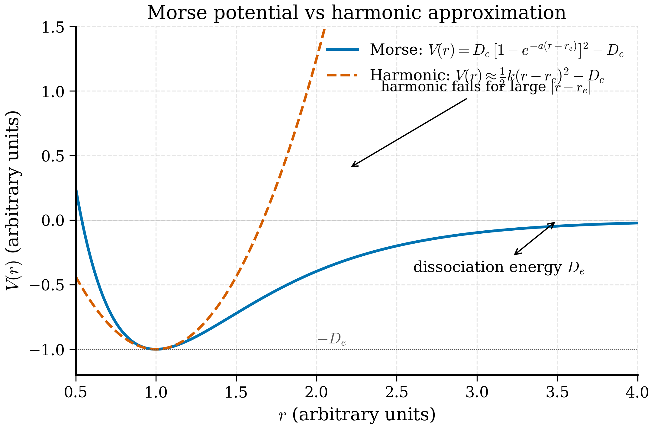
The Morse potential — a paradigmatic anharmonic correction¶

The most popular analytical model for a real chemical bond is the Morse potential,

\[V_{\mathrm M}(r) = D_e\left[1 - e^{-a(r - r_e)}\right]^2, \tag{4.4.M1}\]

where $r_e$ is the equilibrium bond length, $D_e$ is the dissociation energy, and $a$ controls the width of the well. Expanding $V_{\mathrm M}$ about $r = r_e$,

\[V_{\mathrm M}(r) \approx D_e a^2 (r - r_e)^2 - D_e a^3 (r - r_e)^3 + \tfrac{7}{12} D_e a^4 (r - r_e)^4 + \cdots,\]

so the harmonic approximation has $k = 2 D_e a^2$ and $\omega = \sqrt{2 D_e a^2/m}$. The cubic and quartic corrections produce anharmonicity in a controlled way. Remarkably, the Schrödinger equation for the Morse potential is exactly solvable; the energies are

\[E_n = \hbar\omega(n + \tfrac12) - \frac{[\hbar\omega(n + \tfrac12)]^2}{4 D_e}, \tag{4.4.M2}\]

a quadratic correction to the SHO spectrum. The levels are no longer evenly spaced: as $n$ grows, the gaps shrink (the bond softens), and the spectrum terminates at a finite number of bound states (the bond breaks). For H$_2$, $D_e \approx 4.75$ eV and $\hbar\omega \approx 0.55$ eV, giving an anharmonic correction to $E_0$ of about $-0.02$ eV — small but spectroscopically measurable.

The Morse curve is plotted alongside the harmonic approximation in Fig. 4.4.2. The two coincide to about 0.1 Å around the minimum and diverge rapidly thereafter. This is the standard cartoon for "harmonic everywhere near the minimum, breaks down at large amplitude" — and is the conceptual basis for why room-temperature solid mechanics is almost harmonic but thermal expansion, thermal conductivity, and bond dissociation require anharmonic terms.

When to worry about anharmonicity

A useful rule of thumb: the harmonic approximation is reliable when the thermal energy $k_B T$ is less than $\sim 10\%$ of the well depth $D_e$. At room temperature ($k_B T \approx 0.026$ eV), this gives a threshold of $D_e \gtrsim 0.25$ eV — easily satisfied by ordinary covalent bonds ($D_e \sim 4$ eV) but failing for weak intermolecular interactions, hydrogen bonds, and any system near a phase transition.

The harmonic oscillator is therefore the lingua franca of vibrational physics: it is the model we start with, the model whose eigenvalues we report, and the model whose deviations we correct. Solving it by hand (as in §4.4.2) and on the computer (as in §4.4.4) is among the most valuable hours you can spend in this book.

4.4.6a Coherent states: the most classical of quantum states¶

It is sometimes asked: what is the most classical state of a quantum oscillator? A definite-energy eigenstate $|n\rangle$ has zero mean position and momentum, which is hardly classical. The answer, due to Schrödinger and Glauber, is a coherent state $|\alpha\rangle$ — a right-eigenstate of the annihilation operator:

\[\hat a|\alpha\rangle = \alpha|\alpha\rangle, \qquad \alpha \in \mathbb C.\]

In the energy basis,

\[|\alpha\rangle = e^{-|\alpha|^2/2}\sum_{n=0}^\infty \frac{\alpha^n}{\sqrt{n!}}\,|n\rangle.\]

Coherent states have several remarkable properties:

The mean position oscillates exactly as a classical particle: $\langle\hat x(t)\rangle = \sqrt{2}\,x_0\,\text{Re}(\alpha\, e^{-i\omega t})$.
The position and momentum uncertainties saturate the Heisenberg bound: $\Delta x\,\Delta p = \hbar/2$, with $\Delta x = x_0/\sqrt 2$.
The wavepacket does not spread with time — a Gaussian of fixed width that simply translates back and forth.

Coherent states describe the output of a laser, the motion of an ion in a Paul trap, and the macroscopic vibrations of a mechanical oscillator. They are how the classical limit of the harmonic oscillator emerges naturally from the quantum theory.

4.4.7 What's coming¶

We have now solved two single-particle problems analytically and numerically. The wavefunction is a complex function on $\mathbb R$, the Hamiltonian is a tridiagonal matrix, and scipy.linalg.eigh does the rest. It is tempting to imagine that real materials will yield to the same recipe.

They do not. The trouble is that a real material contains many electrons, and many electrons interact with each other. The wavefunction becomes a function not of one coordinate but of all $3N$ coordinates of all $N$ electrons in the system. The Hilbert space grows exponentially with $N$. The next section confronts this catastrophe head-on.