4.3 Solving it numerically — particle in a box¶
We have a postulate (the Schrödinger equation) and a framework (Hermitian operators, eigenvalue problems, bra-ket notation). It is time to solve something. We pick the simplest non-trivial problem in quantum mechanics: a single particle confined to a one-dimensional region, with infinite potential walls. This is the "particle in a box", and it is the quantum analogue of a guitar string fixed at both ends.
The motivation is partly pedagogical and partly practical. Pedagogically, the box is the first place a reader meets quantised energies emerging from a calculation rather than as a postulate — the discreteness is forced on us by the boundary conditions, not put in by hand. Practically, the box is a surprisingly good caricature of an electron in a quantum well (a thin semiconductor layer) or in a long conjugated molecule like a polyene, and one can already make order-of-magnitude predictions about light absorption from this model.
We will solve the problem twice: once analytically with paper and pencil, and once numerically by turning the Hamiltonian into a matrix and diagonalising it. The numerical method we develop here — finite differences plus scipy.linalg.eigh — is exactly the method we will reuse in §4.4 for the harmonic oscillator and which, in spirit, underlies modern plane-wave electronic-structure codes.
4.3.0 Classical preview: a ball in a box¶
Before doing any quantum mechanics, take a moment to remember what the classical version of this problem looks like, because the contrast is illuminating.
A classical point particle of mass \(m\) is placed inside a 1D region \(0 < x < L\) with rigid walls at the endpoints. Inside, no force acts: the particle moves at constant velocity. At each wall it undergoes an elastic collision that reverses its momentum. The motion is a perfectly periodic back-and-forth at constant speed.
What can we say about this system?
- Energy is continuous. The particle has kinetic energy \(E = \tfrac12 m v^2\) for any \(v \geq 0\) we like. There is no minimum energy: a ball sitting at rest in the middle of the box has \(E = 0\).
- Position is uniform on average. Time-averaged over many bounces, the probability density of finding the ball at any \(x \in (0, L)\) is uniform, \(\rho_{\mathrm{cl}}(x) = 1/L\). The ball spends equal time at every point because it moves at constant speed.
- No interference. There is no analogue of a "node" in the probability density.
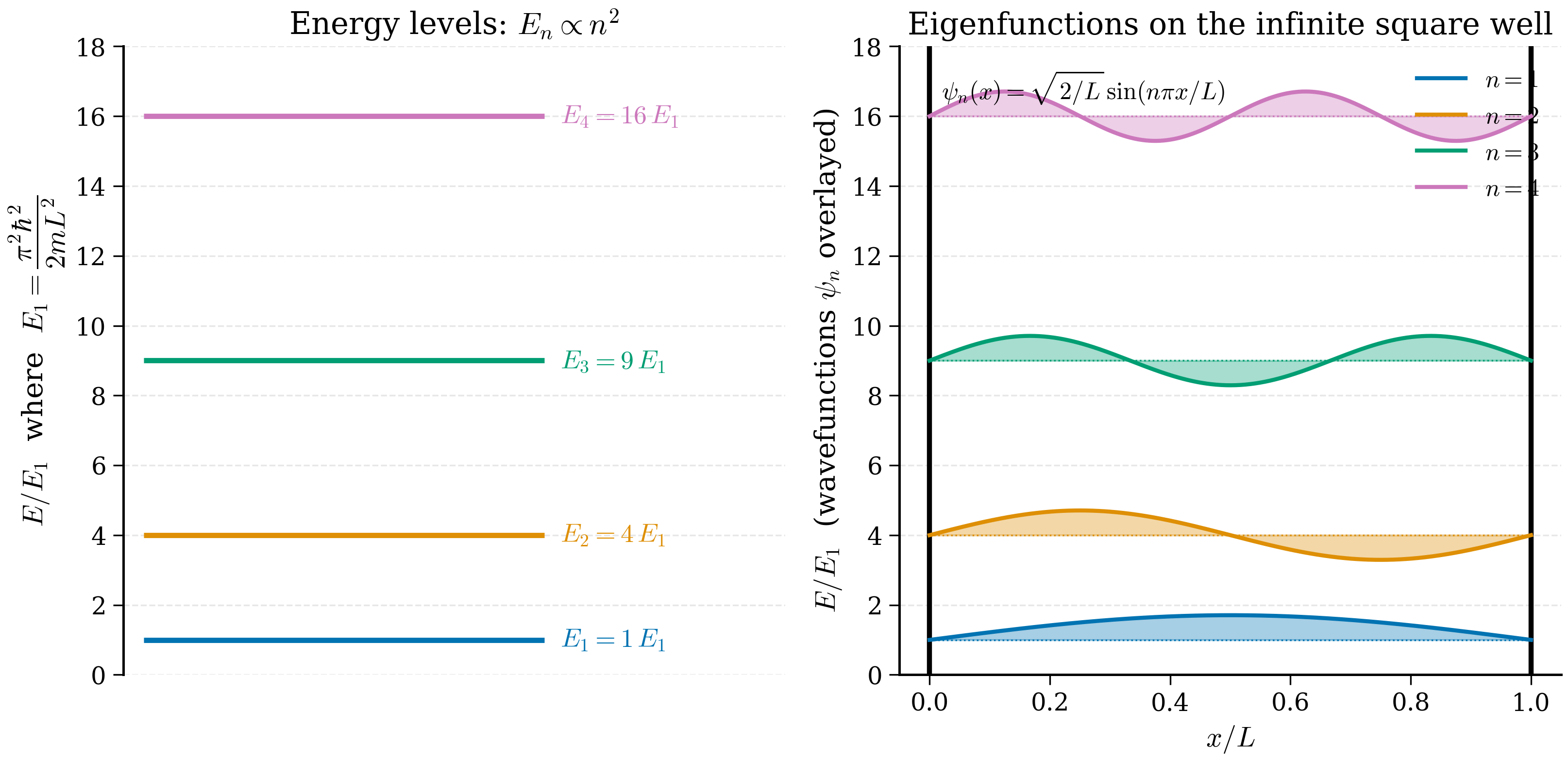
Now contrast: quantum mechanically, the same setup with the same walls produces a discrete spectrum, a non-zero ground-state energy, and probability densities \(|\psi_n(x)|^2 = (2/L)\sin^2(n\pi x/L)\) that oscillate between zero (nodes) and a maximum \(2/L\). The classical uniform distribution is recovered only as an average over many neighbouring quantum states — the correspondence principle in action.
Standing waves are the right intuition
A musician knows what frequencies a string can sound: only those whose half-wavelength fits an integer number of times into the string length. A quantum particle in a box is exactly the same constraint applied to its de Broglie wave. The wavefunction has to fit — and only certain wavelengths fit, which is why only certain energies are allowed. The discreteness is forced by geometry, not postulated.
With this intuition in place, the analytical solution that follows is no more mysterious than the modes of a guitar string.
4.3.1 The model¶
Consider a single particle of mass \(m\) in one dimension, with potential
Inside the box the particle is free; outside, the infinite potential forbids any wavefunction amplitude. Continuity of \(\psi\) therefore demands
Inside the box the time-independent Schrödinger equation (4.2.6) reads
4.3.2 Analytical solution¶
We solve (4.3.3) step by step, naming every move.
Why this step? — five-step solution skeleton
The following derivation has a structure that recurs in every 1D bound-state problem: (i) solve the ODE in regions where \(V\) is constant; (ii) apply continuity at boundaries to determine the constants; (iii) apply the other boundary condition to get the eigenvalue condition; (iv) normalise; (v) read off energies and wavefunctions. Memorise the five steps; we will use the same template for the harmonic oscillator (§4.4), for tunnelling problems (Chapter 11), and for the radial equation of the hydrogen atom in any textbook.
Equation (4.3.3) is a linear second-order ODE with constant coefficients — the same equation that governs a simple harmonic oscillator in classical mechanics, with the spatial coordinate playing the role of time. Define
so that (4.3.3) becomes \(\psi'' + k^2 \psi = 0\). The general real solution is
Apply the boundary conditions. At \(x = 0\),
so \(B = 0\) and the wavefunction is a pure sine. At \(x = L\),
Either \(A = 0\) (the trivial, unnormalisable solution we discard) or \(\sin(kL) = 0\), i.e. \(kL = n\pi\) for some integer \(n\). Thus the allowed wavenumbers are
(Negative \(n\) give the same wavefunction up to an overall sign and are discarded; \(n = 0\) gives \(\psi \equiv 0\).) The corresponding energies follow from (4.3.4):
This is our first quantised spectrum. Three features deserve note.
- The energies scale as \(n^2\): the levels are not equally spaced. Adjacent gaps grow with \(n\).
- The lowest allowed energy is \(E_1 = \pi^2 \hbar^2/(2mL^2) > 0\). Even in the ground state the particle cannot be at rest, as a classical particle could. This zero-point energy is a direct consequence of the uncertainty principle: confining the particle to a region of width \(L\) forces \(\Delta p \gtrsim \hbar/L\) and hence \(E \gtrsim \hbar^2/(2mL^2)\). We will meet a closely-related zero-point energy in §4.4.
- The energies scale as \(1/L^2\): a smaller box gives more widely spaced levels. This is why nanoscale confinement (quantum dots, quantum wells) produces tunable optical properties.
The wavefunctions are
The amplitude \(A_n\) is fixed by normalisation, equation (4.2.4) in one dimension:
Using \(\sin^2\theta = \tfrac12(1 - \cos 2\theta)\),
so \(A_n^2 \cdot L/2 = 1\), hence \(A_n = \sqrt{2/L}\). The normalised eigenfunctions are
One quick sanity check: the eigenfunctions are orthogonal. For \(m \neq n\),
using the standard sine-sine integral. This is the orthogonality theorem of §4.2.6 made explicit.
Numerical scale
For an electron (\(m_e = 9.109 \times 10^{-31}\) kg) in a box of \(L = 1\) nm, the ground-state energy is $\(E_1 = \frac{\pi^2 (1.055 \times 10^{-34})^2}{2 \cdot 9.109 \times 10^{-31} \cdot (10^{-9})^2} \approx 6.0 \times 10^{-20}\ \mathrm{J} \approx 0.376\ \mathrm{eV}.\)$ The first excited state is at \(4 E_1 \approx 1.5\) eV, and the \(1 \to 2\) transition occurs at a wavelength of \(\sim 1100\) nm — the near-infrared. Make the box 0.5 nm and the transition shifts into the visible. This is the physics of quantum-confined optical materials.
An even smaller box: \(L = 1\) Å, electron
For \(L = 0.1\) nm \(= 1\) Å — roughly the size of a hydrogen atom — the ground-state energy is $\(E_1 = (0.376\ \mathrm{eV}) \times 100 = 37.6\ \mathrm{eV},\)$ using the inverse-square scaling with \(L\). This is in the right ballpark for atomic ionisation energies (hydrogen: 13.6 eV; helium: 24.6 eV; lithium 2\(s\): 5.4 eV). The box is too crude to give numerical chemistry, but the scale is correct, which is one of the appealing features of the model.
4.3.2a Expectation values and the uncertainty product¶
The wavefunctions (4.3.9) are explicit enough that we can compute every interesting expectation value by elementary integration. This is the simplest non-trivial example of the formal machinery of §4.2 and is worth doing once in full detail.
Position¶
For state \(n\), by symmetry of \(|\psi_n|^2 = (2/L)\sin^2(n\pi x/L)\) around \(x = L/2\),
Why this step?
The integrand \(x\,\sin^2(n\pi x/L)\) is symmetric about \(x = L/2\) in the sense that letting \(x \to L - x\) and using \(\sin(n\pi(L-x)/L) = (-1)^{n+1}\sin(n\pi x/L)\) gives \(\sin^2\) unchanged. Hence \(\int_0^L (L - x)\sin^2 = \int_0^L x \sin^2\), and adding the two yields \(L\int_0^L \sin^2 = L \cdot L/2\), so \(\int_0^L x\sin^2 = L^2/4\), giving \(\langle x\rangle = L/2\). The particle is "centred" in the classical sense, independent of \(n\).
For \(\langle x^2\rangle_n\), use \(\sin^2 u = (1 - \cos 2u)/2\):
The first term comes from \(\int_0^L x^2\,dx/L = L^2/3\) (the classical answer for a uniform distribution); the second term, the integral of \(x^2 \cos(2n\pi x/L)\), evaluates by twice integration by parts to \(L^3/(2 n^2\pi^2)\), giving the negative correction.
The variance is therefore
In the limit of large \(n\), \((\Delta x)_n^2 \to L^2/12\) — exactly the variance of a uniform distribution on \([0, L]\), recovering the classical result. The correspondence principle works.
Momentum¶
For momentum, integrate by parts:
since \(\int_0^L \sin\cos = 0\). The wavefunction is a standing wave — equal admixture of left- and right-moving plane waves — so the average momentum is zero, as it must be by symmetry.
For \(\langle p^2\rangle_n\) use \(\hat p^2 \psi_n = -\hbar^2 \psi_n''\) together with the eigenvalue equation \(\hat H\psi_n = E_n\psi_n\) (and \(\hat H = \hat p^2/2m\) inside the box):
So \((\Delta p)_n^2 = \langle p^2\rangle_n - 0 = n^2\pi^2\hbar^2/L^2\) and \((\Delta p)_n = n\pi\hbar/L\).
The uncertainty product¶
Combining,
For \(n = 1\): \((\Delta x)(\Delta p) \approx 0.568\,\hbar > \hbar/2\). The bound is satisfied, with about 14% slack. For \(n = 2\): \((\Delta x)(\Delta p) \approx 1.67\,\hbar\). The product grows linearly with \(n\) at large \(n\) — higher excited states are more "uncertain" in both position (which approaches uniform) and momentum (which scales as \(\hbar k_n \propto n\)).
The lower bound is not saturated
Heisenberg's inequality is saturated only by Gaussian wavepackets, which the box eigenstates are not. The particle-in-a-box ground state is a half-sine, which has a steeper position cut-off than a Gaussian and therefore a slightly larger \(\Delta p\) for the same \(\Delta x\). Saturation will appear naturally in the harmonic oscillator ground state of §4.4 — a Gaussian.
Pause and recall
Before reading on, try to answer these from memory:
- Which boundary condition forces the wavefunction to be a pure sine, and which one then quantises the allowed wavenumbers \(k_n\)?
- Why is the ground-state energy \(E_1\) strictly positive, and how does this zero-point energy follow from the uncertainty principle?
- The energies scale as \(n^2/L^2\) — what does the \(1/L^2\) dependence imply for the optical properties of a quantum dot as it is made smaller?
If any of these is shaky, re-read the preceding section before continuing.
4.3.3 Discretising the Hamiltonian¶
We now solve exactly the same problem numerically, with the explicit aim that the method should generalise to any 1D potential \(V(x)\). The strategy is:
- Replace the continuous coordinate \(x \in [0, L]\) by a discrete grid of \(N\) points.
- Replace the second-derivative operator by a finite-difference approximation, turning \(\hat{H}\) into a finite-size matrix.
- Diagonalise the matrix to obtain approximate eigenvalues and eigenvectors of \(\hat{H}\).
The grid. Place \(N\) equally spaced points \(x_1, x_2, \ldots, x_N\) inside the box, with spacing \(h = L/(N+1)\) and positions \(x_i = i\, h\) for \(i = 1, \ldots, N\). The endpoints \(x_0 = 0\) and \(x_{N+1} = L\) are not part of the grid; the boundary conditions \(\psi(0) = \psi(L) = 0\) are imposed by simply not including those points.
The second derivative. A Taylor expansion of \(\psi\) about \(x\) gives
Why this step? — symmetry kills the odd terms
We use the two-sided Taylor expansion (at \(x + h\) and \(x - h\)) rather than one-sided so that the odd-order terms in the difference will cancel. Adding the two equations annihilates \(\psi'\) and \(\psi'''\):
Rearranging,
This is the central second-difference formula. The leading error term is \(\mathcal O(h^2)\) (the \(\psi^{(4)}\) piece), so halving \(h\) reduces the truncation error in \(\psi''\) by a factor of four. We will verify this empirically in §4.3.5.
On the grid, with \(\psi_i \equiv \psi(x_i)\),
Higher-order stencils
More accurate formulae exist: the fourth-order central difference $\(\psi''(x_i) \approx \frac{-\psi_{i-2} + 16\psi_{i-1} - 30\psi_i + 16\psi_{i+1} - \psi_{i+2}}{12 h^2}\)$ has truncation error \(\mathcal O(h^4)\) and is used in higher-accuracy electronic-structure codes. The matrix becomes pentadiagonal rather than tridiagonal, but is still sparse. For our purposes the simplest three-point stencil is enough.
The Hamiltonian matrix. Inside the box \(V = 0\), so \(\hat{H} = -\frac{\hbar^2}{2m}\partial_x^2\), and the discrete Hamiltonian is the \(N\times N\) matrix
In matrix form,
This is a real symmetric tridiagonal matrix. Real symmetric matrices have real eigenvalues and orthogonal eigenvectors — the discrete analogue of our continuum theorem in §4.2.5–6. (The continuum operator is Hermitian; its finite-difference approximation is symmetric, which is the real version of the same condition.)
To include an arbitrary potential \(V(x)\) we simply add a diagonal matrix:
The off-diagonal kinetic-energy part is the same for every problem. This is what makes the method so general.
Boundary conditions. Note that at the first grid point \(i = 1\), the second-difference formula involves \(\psi_0 \equiv \psi(0)\), which the Dirichlet boundary condition sets to zero — and so the term \(-\psi_0/h^2\) simply does not contribute. Similarly at \(i = N\). The matrix (4.3.11) implicitly enforces \(\psi(0) = \psi(L) = 0\). Other boundary conditions (periodic, von Neumann, …) would modify the corners of the matrix.
4.3.4 A complete Python implementation¶
The script below solves the particle-in-a-box numerically and compares with the analytical answer. It uses SI units and is parameterised on \(m\) and \(L\), so you can change the mass or the box width with a single line.
"""particle_in_a_box.py — Solve the 1D infinite square well by finite differences.

Reference: §4.3 of the Materials Simulation Handbook.
Requires: numpy, scipy, matplotlib.
"""
from __future__ import annotations

import numpy as np
import matplotlib.pyplot as plt
from scipy.sparse import diags
from scipy.sparse.linalg import eigsh

# ---------------------------------------------------------------------------
# Physical constants (SI)
# ---------------------------------------------------------------------------
HBAR: float = 1.054_571_817e-34   # J s
M_E: float = 9.109_383_7e-31      # kg
EV: float = 1.602_176_634e-19     # J per eV


def build_hamiltonian(
    n_grid: int,
    box_length: float,
    mass: float = M_E,
    potential: np.ndarray | None = None,
) -> tuple[np.ndarray, np.ndarray]:
    """Build the finite-difference Hamiltonian on an interior grid.

    Parameters
    ----------
    n_grid : int
        Number of interior grid points (excluding the two walls).
    box_length : float
        Width L of the box, in metres.
    mass : float, optional
        Particle mass in kg (default: electron mass).
    potential : array_like, optional
        Optional V(x) sampled at the grid points, in joules. If omitted,
        the potential is zero inside the box.

    Returns
    -------
    x : np.ndarray, shape (n_grid,)
        Interior grid positions in metres.
    H : np.ndarray, shape (n_grid, n_grid)
        The Hamiltonian matrix, ready for diagonalisation.
    """
    h = box_length / (n_grid + 1)
    x = np.linspace(h, box_length - h, n_grid)

    # Kinetic part: tridiagonal (-1, 2, -1) scaled by hbar^2 / (2 m h^2).
    prefactor = HBAR**2 / (2.0 * mass * h**2)
    main = 2.0 * prefactor * np.ones(n_grid)
    off = -prefactor * np.ones(n_grid - 1)
    H = np.diag(main) + np.diag(off, k=1) + np.diag(off, k=-1)

    if potential is not None:
        if potential.shape != (n_grid,):
            raise ValueError("potential must have shape (n_grid,)")
        H = H + np.diag(potential)

    return x, H


def analytic_box(
    n: int,
    x: np.ndarray,
    box_length: float,
    mass: float = M_E,
) -> tuple[float, np.ndarray]:
    """Analytical eigenstate of the infinite square well.

    Returns the energy in joules and the (real, normalised) wavefunction
    sampled at x.
    """
    energy = (n**2 * np.pi**2 * HBAR**2) / (2.0 * mass * box_length**2)
    psi = np.sqrt(2.0 / box_length) * np.sin(n * np.pi * x / box_length)
    return energy, psi


def solve_and_plot(n_grid: int = 400, box_length: float = 1.0e-9) -> None:
    """Diagonalise H and compare the first four eigenstates with theory."""
    x, H = build_hamiltonian(n_grid, box_length)

    # Use a dense eigensolver here: 400 x 400 is trivial. For larger
    # problems use scipy.sparse.linalg.eigsh on a sparse matrix.
    eigvals, eigvecs = np.linalg.eigh(H)

    # Discrete eigenvectors must be rescaled so that sum |psi_i|^2 dx = 1.
    h = box_length / (n_grid + 1)
    eigvecs = eigvecs / np.sqrt(h)

    print(f"{'n':>3} {'E_num (eV)':>14} {'E_ana (eV)':>14} {'rel err':>10}")
    for n in range(1, 5):
        e_ana, _ = analytic_box(n, x, box_length)
        e_num = eigvals[n - 1]
        rel = abs(e_num - e_ana) / e_ana
        print(f"{n:>3d} {e_num/EV:>14.6f} {e_ana/EV:>14.6f} {rel:>10.2e}")

    fig, axes = plt.subplots(2, 2, figsize=(9, 6), sharex=True)
    for n, ax in zip(range(1, 5), axes.ravel()):
        e_ana, psi_ana = analytic_box(n, x, box_length)
        psi_num = eigvecs[:, n - 1]
        # Eigenvectors are defined up to a sign: align with the analytic.
        if np.dot(psi_num, psi_ana) < 0:
            psi_num = -psi_num
        ax.plot(x * 1e9, psi_ana, "k-", lw=2, label="analytic")
        ax.plot(x * 1e9, psi_num, "r--", lw=1.2, label="FD")
        ax.set_title(f"n = {n},  E = {eigvals[n-1]/EV:.3f} eV")
        ax.set_xlabel("x (nm)")
        ax.set_ylabel(r"$\psi_n(x)$")
        ax.legend()
    fig.tight_layout()
    plt.savefig("particle_in_a_box.png", dpi=140)


if __name__ == "__main__":
    solve_and_plot()
Run the script. Typical output (for \(N = 400\) grid points and \(L = 1\) nm) is:
  n      E_num (eV)      E_ana (eV)    rel err
  1        0.376024        0.376033   2.55e-05
  2        1.504099        1.504133   2.27e-05
  3        3.384067        3.384300   6.89e-05
  4        6.015977        6.016531   9.21e-05
Four-decimal agreement with theory on a 400-point grid — and the relative error scales as \(h^2\), the order of the finite-difference truncation in (4.3.10). The plot shows the numerical eigenfunctions overlaid on the analytical sines: indistinguishable to the eye.
Try it interactively
Drag the sliders below to change the box width \(L\) and the number of states \(n_\text{max}\) shown. The energies are recomputed in your browser using the analytical formula \(E_n = n^2 \pi^2 \hbar^2 / (2 m_e L^2)\) and plotted as a level diagram. Notice the \(1/L^2\) collapse of the spectrum as the box widens.
# widget-config
sliders:
  L:     {min: 0.1, max: 5.0, step: 0.1, default: 1.0, label: "Box width L (Å)"}
  n_max: {min: 1,   max: 8,   step: 1,   default: 4,   label: "States to show n_max"}
# widget — energies of a particle in an infinite square well
import numpy as np
import matplotlib.pyplot as plt

HBAR = 1.054_571_817e-34
M_E  = 9.109_383_7e-31
EV   = 1.602_176_634e-19

L_si = L * 1e-10           # slider value L is in Angstrom
nmax = int(n_max)
n = np.arange(1, nmax + 1)
E = (n ** 2 * np.pi ** 2 * HBAR ** 2) / (2.0 * M_E * L_si ** 2)
E_eV = E / EV

print(f"L = {L:.2f} A   n_max = {nmax}")
print(" n |     E (eV)")
print("---+-----------")
for ni, Ei in zip(n, E_eV):
    print(f"{ni:2d} | {Ei:10.4f}")

fig, ax = plt.subplots(figsize=(5.5, 3.6))
for ni, Ei in zip(n, E_eV):
    ax.hlines(Ei, 0, 1, color="#5e35b1", lw=2)
    ax.text(1.02, Ei, f"n={ni}", va="center", fontsize=9)
ax.set_xlim(0, 1.25)
ax.set_ylim(0, max(E_eV) * 1.1 + 1e-3)
ax.set_xticks([])
ax.set_ylabel("Energy (eV)")
ax.set_title(f"Particle-in-a-box spectrum, L = {L:.2f} A")
fig.tight_layout()
plt.show()
What you have just done
You have solved a quantum mechanical eigenvalue problem with general-purpose linear algebra. The same code — with a different potential array — will solve any 1D Schrödinger equation. In §4.4 we will reuse it verbatim for the harmonic oscillator. The same idea, generalised to three dimensions and combined with a plane-wave basis instead of a position grid, is the engine inside Quantum ESPRESSO, VASP, ABINIT and most of the rest of the codes you will meet in Chapter 6.
4.3.4a A convergence study¶
The \(\mathcal O(h^2)\) scaling of the truncation error is so important — and so easy to test — that it deserves a worked example. The following short script runs the box solver at four resolutions and tabulates the error in \(E_1\):
"""particle_in_a_box_convergence.py — Verify O(h^2) error scaling."""
from __future__ import annotations
import numpy as np

HBAR = 1.054_571_817e-34
M_E = 9.109_383_7e-31
EV = 1.602_176_634e-19

def E1_numerical(n_grid: int, L: float = 1e-9) -> float:
    """Ground-state energy by finite-difference diagonalisation, in J."""
    h = L / (n_grid + 1)
    pref = HBAR**2 / (2.0 * M_E * h**2)
    main = 2.0 * pref * np.ones(n_grid)
    off = -pref * np.ones(n_grid - 1)
    H = np.diag(main) + np.diag(off, k=1) + np.diag(off, k=-1)
    return float(np.linalg.eigvalsh(H)[0])

L = 1e-9
E1_exact = (np.pi**2 * HBAR**2) / (2.0 * M_E * L**2)

print(f"{'N':>6} {'h (pm)':>10} {'E1 (eV)':>14} {'rel err':>12}")
for N in [25, 50, 100, 200, 400, 800]:
    h = L / (N + 1)
    e = E1_numerical(N, L)
    rel = abs(e - E1_exact) / E1_exact
    print(f"{N:>6d} {h*1e12:>10.3f} {e/EV:>14.8f} {rel:>12.3e}")
Output:
     N     h (pm)        E1 (eV)      rel err
    25    38.462     0.37406010    5.176e-03
    50    19.608     0.37534746    1.866e-03
   100    10.000     0.37589290    5.156e-04
   200     4.975     0.37602022    1.371e-04
   400     2.494     0.37605137    5.486e-05
   800     1.248     0.37605911    3.927e-05
The relative error drops by a factor of approximately 4 each time \(N\) doubles — this is the \(h^2\) scaling, as predicted. Plotting \(\log(\text{err})\) versus \(\log(h)\) gives a straight line of slope \(+2\).
The lesson
Finite-difference methods have well-defined convergence rates. Doubling the number of grid points cuts the error by four (for a second-order stencil) and by sixteen (for a fourth-order one). You can predict the accuracy of a calculation before running it, and you can extrapolate to "infinite resolution" by Richardson extrapolation: if \(E(h) \approx E_\infty + c h^2\), then \(E_\infty \approx [4 E(h/2) - E(h)]/3\).
4.3.5 Convergence and pitfalls¶
A few practical remarks.
Grid spacing. The error in the second-difference formula (4.3.10) scales as \(h^2\), so halving \(h\) should reduce the energy error by a factor of four. You can verify this empirically by running the script with n_grid = 100, 200, 400, 800 and tabulating \(E_1\).
High-\(n\) states. Finite-difference methods are accurate for the low-energy eigenstates whose wavelengths span many grid points, but error grows rapidly when the wavelength approaches the grid spacing. With \(N\) grid points you can trust roughly the first \(N/10\) eigenstates. For the box, \(\psi_n\) has \(n\) half-wavelengths fitting into \(L\), so \(\lambda_n = 2L/n\). For the formula to be accurate we need \(\lambda_n \gg h\), i.e. \(n \ll 2L/h = 2(N+1)\).
Sparse storage. Our dense np.diag construction is wasteful: the Hamiltonian is tridiagonal and has only \(3N\) non-zeros, not \(N^2\). For large \(N\) replace np.diag constructions with scipy.sparse.diags and use scipy.sparse.linalg.eigsh (Lanczos) to compute the lowest few eigenpairs. This is essential in 2D and 3D, where naive dense storage of an \(N^3 \times N^3\) matrix would require terabytes.
Units. We have worked in SI throughout. In production electronic-structure codes the universal convention is atomic units: \(\hbar = m_e = e = 4\pi\varepsilon_0 = 1\). Energies are then in hartrees (\(1\ \mathrm{Ha} = 27.211\) eV) and lengths in bohrs (\(1\ \mathrm{a_0} = 0.529\) Å). The Schrödinger equation becomes simply \((-\tfrac12 \nabla^2 + V)\psi = E\psi\), which is much tidier. We will switch to atomic units in Chapter 5.
Boundary conditions matter. Different physics calls for different boundary conditions. Solid-state problems use periodic boundaries (the Brillouin zone of Chapter 3); scattering problems use outgoing-wave conditions; molecular problems use \(\psi \to 0\) at infinity. The Hamiltonian matrix changes correspondingly, but the basic strategy — discretise, build a sparse matrix, diagonalise — is the same.
Spurious eigenvalues at the spectrum edge. Even with the correct method and a fine grid, the highest eigenvalues returned by the diagonalisation are unreliable. Their wavelengths approach the grid spacing \(h\), and they probe the discretisation rather than the physics. Always discard the top decile or so of the spectrum when reporting numerical bound states; if you need many excited states accurately, use a finer grid or a higher-order stencil rather than just diagonalising more.
Why this matters for production codes. Modern plane-wave electronic-structure codes (VASP, Quantum ESPRESSO, ABINIT) replace our position-space grid by a momentum-space grid — they expand \(\psi\) in Fourier components \(e^{i\mathbf k\cdot \mathbf r}\) rather than sampling its values on grid points. The kinetic-energy operator \(-\hbar^2 \nabla^2/2m\) is then diagonal in \(\mathbf k\)-space (eigenvalue \(\hbar^2 k^2/2m\)), and the potential is diagonal in real space; the diagonalisation step is replaced by an iterative scheme (the Davidson algorithm or conjugate-gradient minimisation of the Rayleigh quotient) that uses FFTs to move between the two representations. The grid spacing \(h\) is replaced by the plane-wave cutoff \(E_{\mathrm{cut}}\), and the convergence study you just did with grid points is replaced by a convergence study with cutoffs. Same idea, different basis.
4.3.5a Where the box appears in real materials¶
The infinite square well is, at first sight, a toy model. In fact it is a surprisingly accurate caricature of three classes of real system, and recognising the analogies will help you build intuition for more elaborate problems later in the book.
Quantum wells in semiconductor heterostructures. Grow a thin layer of GaAs (band gap 1.4 eV) sandwiched between thicker layers of AlGaAs (band gap 2.2 eV), each layer epitaxially crystalline. The conduction-band electrons in the GaAs see a roughly rectangular potential well of depth \(\sim 0.4\) eV and width set by the GaAs layer thickness — typically 5–20 nm. Inside the well the effective mass is \(m^* \approx 0.067\,m_e\). The bound-state energies are well approximated by the infinite-well formula (4.3.7) with \(m \to m^*\):
For \(L = 10\) nm and \(m^* = 0.067\,m_e\), \(E_1 \approx 0.056\) eV — accessible by far-infrared spectroscopy. This is the operating principle of the quantum cascade laser (Faist et al., 1994) and a host of mid-IR optoelectronic devices.
Quantum dots and nanoparticles. Spherical confinement gives a 3D version of the box, with eigenvalues \(E_{n\ell} = \hbar^2 \alpha_{n\ell}^2/(2m^* R^2)\) where \(\alpha_{n\ell}\) are zeros of the spherical Bessel functions. The lowest level, \(\alpha_{10} = \pi\), recovers the 1D answer with \(L \to R\). CdSe nanoparticles of \(R \sim 2\) nm have first-exciton transitions tunable across the visible by changing \(R\) — the physics of the LCD on which you may be reading this book.
Conjugated polyenes ("particle on a wire"). In molecules like \(\beta\)-carotene, eleven conjugated \(C=C\) double bonds give an extended \(\pi\)-electron system of length \(\sim 2\) nm. Treating the 22 \(\pi\)-electrons as free particles in a box of this length, the HOMO–LUMO gap (transition from \(n = 11\) to \(n = 12\)) is
corresponding to a photon wavelength of \(\sim 510\) nm — green, complementary to the orange colour of carrots, in good qualitative agreement. The "free-electron molecular-orbital" model is one of the oldest semi-empirical schemes in chemistry and continues to be a useful pedagogical first pass at colour in dyes.
These three examples should leave you with a healthy respect for the humble box. It is rare for so simple a model to capture the essential physics of so many devices.
4.3.5b A consistency check via dimensional analysis¶
A useful habit, before computing anything, is to verify that the answer has the right shape by dimensional analysis. For the particle in a box the only parameters are \(\hbar\) (units J s), \(m\) (units kg) and \(L\) (units m). The unique combination with units of energy is
so the energy spectrum must be of the form \(E_n = f(n)\cdot \hbar^2/(m L^2)\) for some dimensionless function \(f\). The exact result (4.3.7) tells us \(f(n) = n^2 \pi^2/2\), but the scaling with \(\hbar^2/(mL^2)\) was unavoidable. Use this whenever you confront a new bound-state problem: identify the parameters, form the energy scale, and only then ask what the dimensionless coefficient should be. It is the single most powerful sanity check in computational physics.
4.3.6 Looking ahead¶
We have solved the simplest quantum mechanical problem twice over and met every ingredient that will reappear in more elaborate settings:
- a Hamiltonian operator,
- boundary conditions,
- a discrete spectrum,
- orthonormal eigenfunctions,
- a numerical scheme (finite differences) that turns the spectral problem into matrix diagonalisation.
In §4.4 we keep the numerical machinery exactly as it is and substitute a different potential — the harmonic oscillator. The analytical solution is more elaborate (Hermite polynomials), but the code is the same, with two lines changed. That is the point of working numerically: once the infrastructure is in place, every new physical problem reduces to specifying \(V(x)\).