3b.6 — Specific Heat: Einstein and Debye¶
Why do the Einstein and Debye models exist?
The puzzle (1819-1900): Dulong and Petit measured the heat capacity of many solids and found a remarkably universal value, \(C_v \approx 3R \approx 25\) J K\(^{-1}\) mol\(^{-1}\) at room temperature. This was beautifully explained by classical equipartition (six quadratic DOFs per atom, each carrying \(k_B T/2\)). But by the late 1800s it was clear that \(C_v\) in fact falls dramatically as \(T \to 0\), and the falloff goes as \(T^3\) in non-magnetic insulators. Classical physics had no explanation: equipartition predicts \(C_v\) should be constant.
Einstein's idea (1907): treat every atom as a quantum harmonic oscillator with a single frequency \(\omega_E\). At low \(T\) (\(k_B T \ll \hbar\omega_E\)), the oscillator sits in its ground state and absorbs no heat. This qualitatively explains why \(C_v \to 0\) at \(T \to 0\) — but quantitatively predicts an exponential falloff, far too steep compared to the experimental \(T^3\) law.
Debye's refinement (1912): the real lattice has not one frequency but a continuous spectrum of frequencies, extending from zero (long-wavelength sound waves) up to a maximum \(\omega_D\) (shortest-wavelength modes). Low-frequency modes are always thermally accessible, even at very low \(T\), and they give the residual heat capacity that scales as \(T^3\). The Debye temperature \(\Theta_D = \hbar\omega_D/k_B\) became the single most useful number for characterising the lattice dynamics of a solid.
The picture to keep: modes with \(\hbar\omega \lesssim k_B T\) are "alive" (thermally excited); modes with \(\hbar\omega \gg k_B T\) are "frozen". As \(T\) drops, modes freeze out one by one starting from the top of the spectrum. The shape of the freeze-out curve depends entirely on the low-frequency density of states. For 3D acoustic phonons with \(g(\omega) \propto \omega^2\), the number of alive modes scales as \(T^3\), giving \(C_v \propto T^3\). For a single Einstein frequency, all modes freeze together when \(T \ll \Theta_E\), giving exponential falloff.
What it buys us: a tractable, accurate framework for computing vibrational free energies and equations of state at finite temperature — the workhorse of high-throughput materials thermodynamics.
"Three peas in a pod; classical, Einstein, and Debye." — paraphrased from any sophomore thermodynamics text
The heat capacity of a solid is the most basic finite-temperature observable, and historically it was the first piece of evidence that something quantum was happening in solids. Dulong–Petit (1819) predicted a temperature-independent molar heat capacity \(C_v = 3R\) — a beautiful consequence of equipartition. By the late 1800s it was clear that \(C_v\) in fact vanishes as \(T\to 0\), and that the experimental scaling \(C_v \propto T^3\) for non-magnetic insulators could not be reconciled with any classical theory.
Einstein (1907) and Debye (1912) provided the resolution by quantising the lattice vibrations. The Einstein model is the simplest possible: a single oscillator frequency per atom. The Debye model adds the crucial ingredient of a distribution of frequencies with linear dispersion at small \(k\) — and reproduces the \(T^3\) law. Both are special cases of the phonon framework of §3b.5, and they remain the simplest tractable approximations for any practical estimate of vibrational free energies in Chapter 8.
Intuition: low-frequency modes are the survivors
The physical mechanism behind the temperature dependence of \(C_v\) is the freezing-out of high-frequency modes. A quantum harmonic oscillator of frequency \(\omega\) has energy spacing \(\hbar\omega\) between levels. To thermally excite it requires \(k_B T \gtrsim \hbar\omega\). So at temperature \(T\), only modes with \(\omega \lesssim k_B T/\hbar\) are populated; modes with \(\hbar\omega \gg k_B T\) sit in their ground state and contribute essentially nothing to \(C_v\). Lowering the temperature, more and more modes drop out of the contributing pool, and \(C_v\) decreases.
The shape of \(C_v(T)\) at low \(T\) is therefore dictated by how many modes have frequencies below \(\omega \sim k_B T/\hbar\). In Einstein's model all modes have the same frequency \(\omega_E\), so once \(T\) drops below \(\Theta_E\) all modes freeze simultaneously and \(C_v\) falls exponentially fast. In Debye's model the modes have a spectrum extending down to \(\omega = 0\), with density \(g(\omega)\propto \omega^2\) at low \(\omega\) — so the number of modes available below \(k_B T/\hbar\) grows as \(T^3\), and each of those contributes \(\sim k_B\), giving the famous \(T^3\) law. The dimensional analysis is brutal and easy: in \(d\) spatial dimensions with linear dispersion, \(g(\omega)\propto \omega^{d-1}\) at low \(\omega\), and integrating gives \(C_v\propto T^d\) at low \(T\).
3b.6.1 Classical baseline: Dulong–Petit¶
Consider \(N\) atoms, each oscillating in 3D about its equilibrium position. In the harmonic approximation, each atom contributes three independent harmonic oscillators. By the classical equipartition theorem, each quadratic degree of freedom in the Hamiltonian carries \(\tfrac12 k_B T\) of mean energy.
Why this step? — equipartition unpacked
The Hamiltonian of a single harmonic oscillator is \(H = p^2/(2m) + \tfrac12 m\omega^2 x^2\) — quadratic in both \(p\) and \(x\), giving two quadratic degrees of freedom. Classical equipartition says: for any term in \(H\) of the form \(\alpha y^2\), the mean energy at temperature \(T\) is \(\langle\alpha y^2\rangle = \tfrac12 k_B T\), independent of \(\alpha\). (The proof: write the canonical partition function \(Z = \int e^{-\beta\alpha y^2}\,dy = \sqrt{\pi/\beta\alpha}\), hence \(\langle\alpha y^2\rangle = -\partial\ln Z/\partial\beta = 1/(2\beta) = k_B T/2\).) So each oscillator contributes \(k_B T\) from its kinetic part and \(k_B T\) from its potential part — wait, that gives \(k_B T\) total per oscillator, not \(2\cdot k_B T/2\). Let me recheck: kinetic = \(k_B T/2\), potential = \(k_B T/2\), sum = \(k_B T\). So each oscillator (one degree of freedom in real space) carries \(k_B T\), and a 3D atom (three oscillators, one per Cartesian direction) carries \(3 k_B T\). Counting \(N\) atoms gives \(3 N k_B T\), in agreement with the formula below.
For an atom in a 3D harmonic well, there are three oscillators (one per direction) each with two quadratic DOFs (kinetic + potential), for a total of six quadratic DOFs per atom, hence \(6\cdot k_B T/2 = 3 k_B T\) per atom:
Alternatively phrased: 3 translational kinetic DOFs + 3 potential (vibrational) DOFs per atom, \(k_B T/2\) each, total \(3 k_B T\) per atom. So
Differentiating with respect to \(T\),
Empirically this holds at high temperatures (room temperature is "high" for most metals), to within a few percent. At low temperatures, however, \(C_v\) measurably drops far below \(3R\) and tends to zero. Equipartition fails. The reason is that quantum mechanics suppresses the population of high-frequency modes whose excitation energies are large compared to \(k_B T\). Mode by mode this is the harmonic-oscillator energy from Chapter 4. We need to put it back into the sum over modes.
3b.6.2 Einstein model¶
Einstein's idea: assume every atom is an independent harmonic oscillator of the same frequency \(\omega_E\), in three dimensions. The total energy of \(N\) atoms (i.e. \(3N\) oscillators) at temperature \(T\) is
The mean energy of a single quantum harmonic oscillator at temperature \(T\) is
Why this step? — derivation of \(\langle E\rangle_\text{1 osc}\)
For a quantum harmonic oscillator with energy levels \(E_n = \hbar\omega(n + 1/2)\) for \(n = 0, 1, 2, \ldots\), the partition function is $\(Z = \sum_{n=0}^\infty e^{-\beta E_n} = e^{-\beta\hbar\omega/2}\sum_{n=0}^\infty e^{-n\beta\hbar\omega} = \frac{e^{-\beta\hbar\omega/2}}{1 - e^{-\beta\hbar\omega}}.\)$ Then \(\langle E\rangle = -\partial\ln Z/\partial\beta\). After a few lines: $\(\langle E\rangle = \frac{\hbar\omega}{2} + \frac{\hbar\omega\, e^{-\beta\hbar\omega}}{1 - e^{-\beta\hbar\omega}} = \frac{\hbar\omega}{2} + \frac{\hbar\omega}{e^{\beta\hbar\omega} - 1},\)$ recovering (3b.6.4). The second term is the Bose–Einstein occupation \(n_B(\omega) = 1/(e^{\beta\hbar\omega} - 1)\) multiplied by \(\hbar\omega\) — exactly the average thermal excitation in units of \(\hbar\omega\).
(The zero-point contribution \(\hbar\omega/2\) does not depend on \(T\) and drops out of \(C_v\).) Differentiating with respect to \(T\),
Why this step? — taking the temperature derivative
Let \(x = \hbar\omega/k_B T = \beta\hbar\omega\). Then \(\langle E\rangle - \hbar\omega/2 = \hbar\omega/(e^x - 1)\). Differentiate w.r.t. \(T\): \(dx/dT = -x/T\). So $\(\frac{d}{dT}\frac{\hbar\omega}{e^x - 1} = -\frac{\hbar\omega\, e^x}{(e^x-1)^2}\cdot\frac{dx}{dT} = \frac{\hbar\omega\, e^x}{(e^x-1)^2}\cdot\frac{x}{T} = k_B x^2\cdot\frac{e^x}{(e^x-1)^2},\)$ which is exactly (3b.6.5).
Summing over all \(3N\) oscillators,
Define the Einstein temperature \(\Theta_E := \hbar\omega_E/k_B\). The high- and low-\(T\) limits:
High \(T\) (\(T\gg \Theta_E\)). \(e^x \approx 1 + x\), so \((e^x - 1)^2 \approx x^2\) and \(e^x \approx 1\). Substituting,
recovering Dulong–Petit. Good.
Low \(T\) (\(T\ll \Theta_E\)). Let \(x = \Theta_E/T \gg 1\). Then \(e^x \gg 1\), so \((e^x - 1)^2 \approx e^{2x}\) and the numerator \(e^x\) gives a ratio \(e^x/e^{2x} = e^{-x}\). Hence
The Einstein heat capacity drops exponentially with \(1/T\). Experimentally, however, \(C_v\propto T^3\) in real insulators, which is a power-law falloff, vastly slower than exponential. Einstein's model decays much too fast.
How fast is 'much too fast'? — a numerical comparison
Take \(\Theta_E = 300\) K (typical for many simple solids), and consider \(T = 30\) K, i.e. \(T/\Theta_E = 0.1\) and \(\Theta_E/T = 10\). Einstein prediction: $\(C_v / (3Nk_B) \approx (10)^2\cdot e^{-10} \approx 100\cdot 4.5\times 10^{-5} \approx 4.5\times 10^{-3}.\)$ Debye prediction (with \(\Theta_D = 300\) K, using the \(T^3\) law): $\(C_v/(3Nk_B) \approx \frac{12\pi^4}{5}\cdot (0.1)^3/3 \approx 77.9\cdot 0.001/3 \approx 0.026.\)$ Wait, let me recheck the Debye factor: \(12\pi^4/5 \approx 233.8\), and \((T/\Theta_D)^3 = 0.001\), so \(C_v/(Nk_B) \approx 0.234\), i.e. \(C_v/(3Nk_B) \approx 0.078\). The Debye value is about 17 times larger than the Einstein value at \(T = 0.1\,\Theta\). The discrepancy widens rapidly as \(T\) drops further: at \(T = 0.05\,\Theta\), Einstein gives \(\sim 10^{-7}\) while Debye gives \(\sim 10^{-2}\) — a five-decade gap. The Einstein model is therefore qualitatively useless below about \(\Theta/3\).
The reason for the discrepancy is physically obvious in retrospect. By collapsing all modes to a single frequency \(\omega_E\), Einstein excised the existence of arbitrarily low-frequency modes — long-wavelength acoustic phonons with \(\omega\to 0\) as \(k\to 0\). These low-frequency modes are always populated, even at very low \(T\), and their contribution falls off only as a power of \(T\). To capture them you need a distribution of frequencies extending all the way down to zero. That distribution is what Debye supplied.
When the Einstein model is still useful
For optical phonon branches — high-frequency modes with weak dispersion — the Einstein model is a fine approximation. In a real solid you might use Debye for the acoustic branches and Einstein for each optical branch, with separate \(\Theta_E\) values. This composite approximation is good enough for back-of-envelope free-energy estimates in Chapter 8.
Where does (3b.6.6) come from? — full Einstein derivation¶
Let us assemble (3b.6.6) explicitly. Start from (3b.6.3) and (3b.6.4). The thermal part of the energy of \(3N\) Einstein oscillators (dropping the zero-point) is
The heat capacity is \(C_v = (\partial U_\text{th}/\partial T)_V\). Letting \(x = \hbar\omega_E/k_B T = \Theta_E/T\), \(dx/dT = -x/T\), and using \(d(1/(e^x-1))/dx = -e^x/(e^x-1)^2\),
This is (3b.6.6) with \(x = \Theta_E/T\).
3b.6.3 Debye model¶
Debye's idea: replace the actual phonon spectrum with an isotropic one with strictly linear dispersion \(\omega(\mathbf k) = c_s |\mathbf k|\), valid up to a cutoff wavevector \(k_D\) chosen so that the total number of modes is correct. There are three acoustic branches (the longitudinal and two transverse), and we (Debye, originally) average their sound velocities into a single \(c_s\).
The total number of modes in a crystal of \(N\) atoms is \(3N\). In the Debye model the number of mode in a sphere of radius \(k_D\) is
giving
The Debye frequency and Debye temperature are
Why this step? — Debye sphere mimics the free-electron Fermi sphere
The Debye construction is mathematically isomorphic to the free-electron Fermi sphere of §3b.4. There, electrons fill a sphere in \(\mathbf k\)-space of radius \(k_F\) chosen so the total filled count equals \(N_e\). Here, phonons fill a sphere of radius \(k_D\) chosen so that the mode count equals \(3N_\text{at}\) (three branches per atom). The only difference is the factor of three for the three acoustic polarisations. Both spheres define a maximum wavevector beyond which the model has no states.
The phonon density of states in the Debye model is, by direct calculation analogous to (3b.4.10),
Verify normalisation: \(\int_0^{\omega_D} g(\omega) d\omega = V\omega_D^3/(2\pi^2 c_s^3) = V k_D^3/(2\pi^2) = 3N\). Good.
The total vibrational energy at temperature \(T\) is
Drop the zero-point part (constant in \(T\)). Substitute \(x = \hbar\omega/k_B T\), \(x_D = \hbar\omega_D/k_B T = \Theta_D/T\):
Using \(V/(c_s^3) = 6\pi^2 N/\omega_D^3\) via (3b.6.10) and (3b.6.11),
Differentiating with respect to \(T\), after some standard manipulations (differentiate the upper limit of the integral, then split — see exercises),
This is the Debye formula. The integral cannot be evaluated in closed form but is easily computed numerically.
High \(T\) (\(T\gg \Theta_D\)). Then \(\Theta_D/T \ll 1\) so the integration range is small and the integrand \(\approx x^4/(x)^2 \cdot 1 = x^2\) (using \(e^x - 1 \approx x\)). The integral \(\approx (\Theta_D/T)^3/3\). So
Dulong–Petit, as required.
Low \(T\) (\(T\ll \Theta_D\)). Then \(\Theta_D/T \gg 1\) and we extend the upper limit to infinity (the integrand is exponentially suppressed beyond \(x\sim 1\), so the extension introduces only exponentially small error). The integral becomes the dimensionless number
Why this step? — evaluating the dimensionless integral
Use integration by parts: let \(u = x^4\) and \(dv = e^x/(e^x-1)^2\, dx\). Then \(du = 4x^3\, dx\) and \(v = -1/(e^x-1)\). So $\(\int_0^\infty \frac{x^4 e^x}{(e^x-1)^2}dx = \left[-\frac{x^4}{e^x-1}\right]_0^\infty + 4\int_0^\infty\frac{x^3}{e^x-1}dx.\)$ The boundary term vanishes at both endpoints (at \(x=0\), \(x^4 \to 0\) faster than \(1/(e^x-1)\sim 1/x\) diverges; at \(x=\infty\), \(1/(e^x-1)\) decays exponentially). The remaining integral is one of the most famous in physics: $\(\int_0^\infty\frac{x^3}{e^x-1}dx = \Gamma(4)\zeta(4) = 6\cdot\frac{\pi^4}{90} = \frac{\pi^4}{15}.\)$ Hence the full integral is \(4\pi^4/15\). The same integral arises in Planck's blackbody radiation law (Stefan–Boltzmann constant) — the Debye \(T^3\) law and the Stefan–Boltzmann \(T^4\) law are two faces of the same mathematics.
So
This is the celebrated Debye \(T^3\) law, confirmed experimentally to high precision in every non-magnetic insulator at temperatures below \(\sim \Theta_D/10\).
The \(T^3\) scaling has a transparent physical origin. At temperature \(T\), modes with \(\hbar\omega \lesssim k_B T\) are thermally populated; modes above this cutoff are frozen. The number of populated modes is the volume in \(\mathbf k\)-space of the sphere \(|\mathbf k| \lesssim k_B T/(\hbar c_s)\), namely \(\propto T^3\). Each populated mode contributes of order \(k_B\) to the heat capacity. So \(C_v\propto T^3\). The same argument in \(d\) dimensions gives \(C_v\propto T^d\).
Debye temperatures across the periodic table¶
The Debye temperature \(\Theta_D\) encodes the stiffness of a lattice: high \(\Theta_D\) means strong bonds and/or light atoms, low \(\Theta_D\) means soft bonds and/or heavy atoms. A representative sampling:
| Material | \(\Theta_D\) (K) | Comment |
|---|---|---|
| Diamond (C) | 2230 | Lightest atom + strongest bonds in nature |
| Beryllium (Be) | 1440 | Light atom, strong covalent character |
| Aluminium (Al) | 428 | Typical sp metal |
| Copper (Cu) | 343 | Typical d-block metal |
| Iron (Fe) | 470 | Magnetic, but lattice still soft enough |
| Silver (Ag) | 225 | Heavier than Cu, softer |
| Gold (Au) | 165 | Heavy and soft |
| Lead (Pb) | 105 | Heavy, very weak bonds |
| Cesium (Cs) | 38 | Heaviest alkali, weakest bonds |
The factor of \(\sim 60\) spread is set largely by atomic mass (a factor of \(\sim 25\) from C to Cs) and by bond strength (another factor of \(\sim 3\)). The Debye frequency scales as \(\sqrt{K/M}\) where \(K\) is bond stiffness and \(M\) is atomic mass; the trends above are quantitatively rationalised by this scaling.
The Debye temperature is also a useful estimator of the temperature below which quantum effects in lattice dynamics matter. For diamond at room temperature, \(T/\Theta_D \approx 0.13\) — the lattice is quantum-mechanically rigid and classical MD overcounts heat capacity by a factor of 2. For lead at room temperature, \(T/\Theta_D \approx 2.9\) — the lattice is firmly classical and Dulong-Petit is accurate. For copper at room temperature, \(T/\Theta_D \approx 0.87\) — quantum corrections are 10–20%. This is precisely the regime where the Debye integral (3b.6.16) is needed rather than its asymptotic limits.
3b.6.4 Comparing models¶
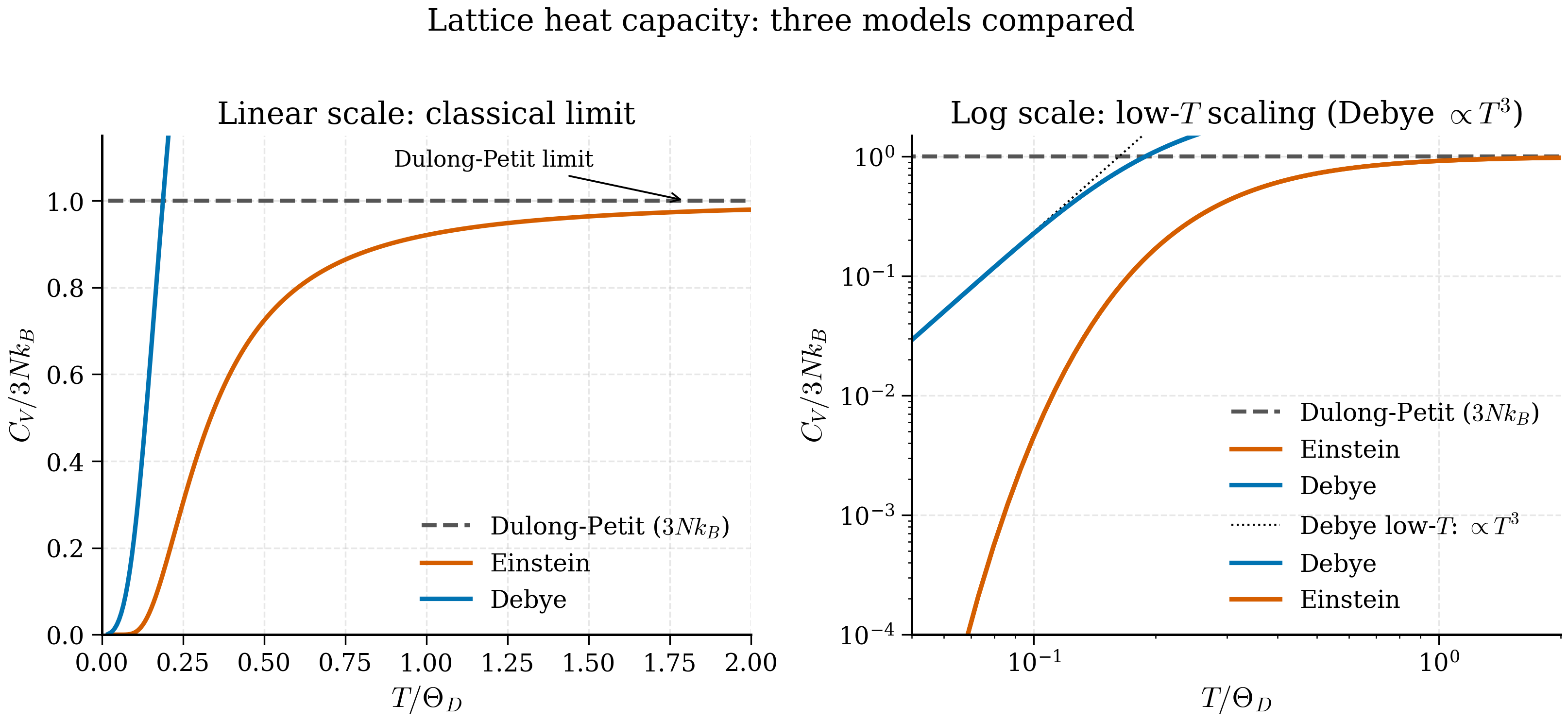
The plot below (you will reproduce it in exercise 3b.8.4) compares \(C_v(T)\) from the three models for a representative material with \(\Theta_D = \Theta_E = 300\) K. All three agree at high \(T\) on the Dulong–Petit value \(3Nk_B\). As \(T\) decreases:
- Classical (Dulong–Petit): flat at \(3Nk_B\) — wrong below room temperature.
- Einstein: drops exponentially below \(\Theta_E\) — wrong at low \(T\), but adequate near and above \(\Theta_E\).
- Debye: drops as \(T^3\) at low \(T\) — matches experiment for acoustic-dominated solids.
In a real material, \(\Theta_D\) ranges from \(\sim 80\) K for soft metals like Pb (heavy atoms, weak bonds) to \(\sim 2200\) K for diamond (light atoms, strong bonds). The Debye temperature is, in fact, the most useful single number for characterising a material's lattice dynamics — it sets the temperature scale below which quantum effects in nuclear motion become important, and it controls the low-temperature heat capacity to a power of 3.
3b.6.5 Numerical evaluation: copper¶
The experimental Debye temperature of copper is \(\Theta_D \approx 343\) K. Let us compute \(C_v^\text{Debye}(T)\) at several temperatures to map out the curve.
\(T = 10\) K (\(T/\Theta_D = 0.0292\), deep in the \(T^3\) regime): $\(C_v/(Nk_B) \approx \frac{12\pi^4}{5}(0.0292)^3 \approx 233.8 \cdot 2.48\times 10^{-5} \approx 5.81\times 10^{-3},\)$ $\(C_v \approx 5.81\times 10^{-3}\, R \approx 0.0483 \text{ J K}^{-1}\text{ mol}^{-1}.\)$ Adding the electronic contribution \(\gamma T \approx 7\times 10^{-4} \cdot 10 = 7\times 10^{-3}\) J K\(^{-1}\) mol\(^{-1}\) — comparable to the lattice part at this low temperature, as expected for a metal near the cross-over.
\(T = 50\) K (\(T/\Theta_D = 0.146\), still in the \(T^3\) regime by (3b.6.19), with \(T/\Theta_D = 0.146\)):
So a mole of copper at 50 K has \(C_v \approx 0.726 R \approx 6.03\) J K\(^{-1}\) mol\(^{-1}\), compared to the Dulong–Petit \(3R \approx 24.9\). About a quarter of the classical value, well below room temperature. Experimentally the heat capacity of copper at 50 K is roughly 6.5 J K\(^{-1}\) mol\(^{-1}\) — agreement to within 8%, the discrepancy ascribed (correctly) to the electronic specific heat from §3b.4 and to deviations from the Debye approximation (the real phonon DOS is not exactly \(\omega^2\)).
\(T = 100\) K (\(T/\Theta_D = 0.292\), the \(T^3\) law starts to break down): the full Debye integral (3b.6.16) gives \(C_v/(Nk_B) \approx 1.81\), i.e. \(C_v \approx 15.0\) J K\(^{-1}\) mol\(^{-1}\) — about 60% of Dulong–Petit. Experimentally \(\approx 16.0\) J K\(^{-1}\) mol\(^{-1}\).
\(T = 300\) K (\(T/\Theta_D = 0.875\), approaching the classical limit): the full Debye integral gives \(C_v/(Nk_B) \approx 2.86\), i.e. \(C_v \approx 23.8\) J K\(^{-1}\) mol\(^{-1}\) — within 5% of Dulong–Petit. Experimentally \(\approx 24.4\) J K\(^{-1}\) mol\(^{-1}\).
The Debye model is therefore quantitatively accurate to within 5–10% across two decades of temperature for a simple monatomic metal like copper. For complex insulators with multiple atoms per cell, the deviations from Debye are larger (optical modes need separate Einstein treatment), but the Debye temperature remains the most useful single number for back-of-envelope free-energy estimates.
For a Python evaluation, the script in exercise 3b.8.4 computes the integral (3b.6.16) numerically by scipy.integrate.quad and plots \(C_v(T)/3Nk_B\) from \(T = 0.01 \Theta_D\) to \(T = 5\Theta_D\). The Dulong–Petit limit is approached from below, and the \(T^3\) law is visible as a straight line on a log-log plot at low \(T\).
Debye derivation of \(C_v\) from first principles — the full chain¶
For completeness, here is the Debye derivation laid out so every step is explicit.
Step 1: The Debye phonon DOS is \(g(\omega) = (3V/(2\pi^2 c_s^3))\,\omega^2\) for \(\omega\le\omega_D\). (Three branches, isotropic linear dispersion.)
Step 2: Thermal internal energy: $\(U_\text{th}(T) = \int_0^{\omega_D} g(\omega)\cdot\frac{\hbar\omega}{e^{\hbar\omega/k_BT}-1}\, d\omega.\)$
Step 3: Substitute \(x = \hbar\omega/k_BT\) (so \(d\omega = (k_BT/\hbar)\,dx\)), and \(\omega = (k_BT/\hbar)\, x\): $\(U_\text{th} = \frac{3V}{2\pi^2 c_s^3}\cdot\frac{(k_BT)^4}{\hbar^3}\int_0^{x_D}\frac{x^3}{e^x-1}\,dx,\)$ with \(x_D = \Theta_D/T\).
Step 4: Eliminate \(V/c_s^3\) via \(\omega_D^3 V/(6\pi^2) = N\) from (3b.6.9)-(3b.6.10), giving \(V/c_s^3 = 6\pi^2 N/\omega_D^3\): $\(U_\text{th} = 9 N k_B T \left(\frac{T}{\Theta_D}\right)^3\int_0^{x_D}\frac{x^3}{e^x-1}\,dx.\)$
Step 5: \(C_v = dU_\text{th}/dT\). Two pieces: differentiating the prefactor \(T^4\) and differentiating the upper limit \(x_D = \Theta_D/T\) (chain rule, \(dx_D/dT = -\Theta_D/T^2\)).
After standard manipulations (the dominant contribution comes from differentiating the integrand factor \(T\) through the integration variable), one arrives at (3b.6.16). The factor-of-3 manipulation between \(T^3\)-law coefficients \(12\pi^4/5\) and the prefactor \(9\) in \(U_\text{th}\) comes from differentiation: \(d/dT(T^4) = 4T^3\), and after combining with the constant \(9\) and the integral value \(\pi^4/15\), one gets \(9\cdot 4\cdot \pi^4/15 = 12\pi^4/5\).
3b.6.6 Beyond Einstein–Debye: realistic phonon DOS¶
In a real material the phonon DOS is computed from the full dynamical matrix (§3b.5), not approximated as \(\omega^2\) up to a cutoff. The vibrational free energy in the harmonic approximation is
The first term is the zero-point energy; the second is the thermal contribution. From \(F\) one obtains \(C_v = -T\partial^2 F/\partial T^2\) and, if the lattice constant is allowed to depend on \(T\), the Helmholtz free energy required for thermal expansion calculations. All of this is the subject of §8.2.
The Debye approximation enters Chapter 8 as a useful sanity check and as a back-of-envelope estimator of vibrational free energy when full phonon spectra are unavailable. For example, to a first approximation, an MLIP that gets the elastic constants right will get \(\Theta_D\) right, which in turn fixes the vibrational entropy of the material to within \(\sim 10\%\). This is sometimes the difference between predicting that a metastable phase is thermodynamically stable above 500 K and not.
Don't trust Debye outside its regime
The Debye \(T^3\) law is exact only in the limit \(T \to 0\) for purely acoustic systems. As soon as \(T\) approaches a fraction of \(\Theta_D\), deviations of the real DOS from \(\omega^2\) matter. Plotting \(C_v/T^3\) vs \(T\) on log axes is the standard diagnostic — flat at low \(T\) (in the Debye regime), then rising as optical modes turn on. The point of departure from flatness is a useful empirical lower bound on the lowest optical phonon frequency.
Worked example: copper at multiple temperatures from full Debye¶
For copper with \(\Theta_D = 343\) K, evaluate the full Debye integral at several temperatures (numerically in your head from the asymptotic limits at extremes, exactly via scipy in the middle):
| \(T\) (K) | \(T/\Theta_D\) | Regime | \(C_v/(3Nk_B)\) | \(C_v\) (J K\(^{-1}\) mol\(^{-1}\)) |
|---|---|---|---|---|
| 10 | 0.029 | \(T^3\) asymptotic | \(\sim 0.0019\) | \(\sim 0.047\) |
| 50 | 0.146 | \(T^3\) regime breaks down | \(\sim 0.242\) | \(\sim 6.0\) |
| 100 | 0.292 | Crossover | \(\sim 0.604\) | \(\sim 15.0\) |
| 150 | 0.437 | Approaching classical | \(\sim 0.787\) | \(\sim 19.6\) |
| 200 | 0.583 | Mostly classical | \(\sim 0.881\) | \(\sim 21.9\) |
| 300 | 0.875 | Almost classical | \(\sim 0.953\) | \(\sim 23.8\) |
| 500 | 1.458 | Classical | \(\sim 0.984\) | \(\sim 24.5\) |
| 1000 | 2.915 | Strictly classical | \(\sim 0.996\) | \(\sim 24.8\) |
The approach to the Dulong-Petit limit \(3Nk_B = 24.94\) J K\(^{-1}\) mol\(^{-1}\) is monotonic from below, reaching 95% at \(T \approx \Theta_D\) and 99% at \(T \approx 3\Theta_D\). The deviation from Dulong-Petit at any single temperature is captured by the single number \(\Theta_D\), which is why \(\Theta_D\) is the most useful single descriptor of a material's lattice dynamics.
Comparing to experimental Cu heat capacity (mostly from low-temperature calorimetry studies), the Debye prediction is accurate to 5-10% across the entire range, with deviations attributable to (i) the electronic contribution \(\gamma T\) from §3b.4, which dominates below ~10 K; (ii) anharmonic effects above ~\(\Theta_D/2\); and (iii) departures of the real Cu phonon DOS from the idealised \(\omega^2\) Debye spectrum.
3b.6.7 The total heat capacity of a real metal¶
In a real metal, the total low-temperature specific heat combines the electronic linear term (§3b.4.7) and the lattice \(T^3\) term:
The standard experimental procedure: measure \(C_v\) at temperatures of a few Kelvin, plot \(C_v/T\) vs \(T^2\); the intercept is \(\gamma\) and the slope is the \(T^3\) coefficient. From the slope one extracts \(\Theta_D\). From \(\gamma\) one extracts \(g(\varepsilon_F)\), which is a quantity that DFT computes natively. So a low-temperature heat-capacity measurement is one of the most direct experimental tests of both the electronic DOS and the phonon DOS predicted by a first-principles calculation. We will return to this in Chapter 6, where you will compute \(\gamma\) and \(\Theta_D\) for a metal and compare to tabulated experimental values.
3b.6.8 Section summary¶
Key ideas
- Dulong-Petit (classical). \(C_v = 3Nk_B\) — six quadratic DOFs per atom by equipartition. Correct at high \(T\); fails at low \(T\) where experiment gives \(C_v \to 0\).
- Einstein (1907). All atoms oscillate at one frequency \(\omega_E\). Predicts \(C_v \to (\Theta_E/T)^2 e^{-\Theta_E/T}\) at low \(T\) — exponentially small, but in fact too fast a falloff vs. experiment's \(T^3\).
- Debye (1912). Replace true phonon spectrum with linear-dispersion approximation \(\omega = c_s k\) up to cutoff \(k_D = (6\pi^2 n)^{1/3}\). Phonon DOS \(g(\omega)\propto\omega^2\). Predicts \(C_v \to (12\pi^4/5) Nk_B(T/\Theta_D)^3\) at low \(T\) — the correct \(T^3\) law.
- Crossover. At \(T \sim \Theta_D\), \(C_v\) approaches Dulong-Petit from below. The Debye temperature \(\Theta_D\) is the most useful single characterisation of a material's lattice dynamics.
- Total \(C_v\) in metals. Electronic linear term + lattice \(T^3\) term: \(C_v = \gamma T + (12\pi^4/5)Nk_B(T/\Theta_D)^3\). Plotting \(C_v/T\) vs. \(T^2\) separates them.
- Beyond Debye. Real materials need full phonon DOS; vibrational free energy from \(\int g(\omega)\ln(2\sinh(\hbar\omega/2k_BT))\,d\omega\) — basis of Ch 8 free energy calculations.
What to remember three months from now: "Heat capacity is a story about which vibrational modes are thermally accessible. Below the Debye temperature, the \(\omega^2\) phonon DOS gives \(C_v\propto T^3\). Above, classical equipartition gives Dulong-Petit. The crossover is at \(T\sim\Theta_D\)."
Where this is used later¶
- Tier 1. §6.6 (Debye temperature from elastic constants — a quick consistency check on a phonon calculation), §6.8 (electronic and lattice contributions to total \(C_v\) at low \(T\)).
- Tier 2. §8.2 (harmonic vibrational free energy, with Debye and Einstein as analytic shortcuts), §8.3 (thermal expansion in the quasi-harmonic approximation), §8.5 (phase stability boundaries set by free-energy differences with vibrational entropy). §9.7 (MLIP benchmarks: matching \(\Theta_D\) within \(\sim 5\%\) is a sine qua non).
- Capstone Project 3. Estimating the operating-temperature stability of a candidate thermoelectric: the vibrational entropy difference between competing phases is computed from Debye temperatures derived from MLIP phonon calculations.
Next: §3b.7 examines what happens when the perfect periodicity is broken — by defects, impurities, and strain — which is, after all, where the interesting physics of real materials lives.