3.4 Reciprocal Space Without Tears
Reciprocal space is the natural setting in which to describe waves moving through a periodic crystal. It is the home of Brillouin zones, \(\mathbf{k}\)-points, band structures, phonon dispersions, and X-ray diffraction patterns. It is also, for many newcomers, the first part of solid-state physics that feels genuinely abstract: an entire space whose points are not positions in the crystal but wavenumbers, used to label labels of basis functions.
This section is an attempt to demystify reciprocal space without burying it in formalism. The mathematics will be precise but light. By the end you should be able to write down the reciprocal-lattice vectors of any crystal you have constructed, sketch its Brillouin zone in the simple cases, and explain why band-structure plots run along peculiar one-dimensional paths through it.
Why reciprocal space exists
The starting point is a single mathematical fact: a function defined on a periodic lattice has a natural Fourier expansion in terms of plane waves whose wavevectors live on a dual lattice — the reciprocal lattice. We saw the one-dimensional version in Chapter 0: a function periodic with period \(L\) is naturally expanded in Fourier components \(e^{i k_n x}\) with \(k_n = 2\pi n / L\). The wavenumbers \(k_n\) form a one-dimensional reciprocal lattice with spacing \(2\pi / L\).
In three dimensions, with a general crystal lattice, the same logic applies, but the reciprocal lattice is also three-dimensional and its geometry depends on the direct-lattice geometry. Any function \(f(\mathbf{r})\) that is periodic on the direct lattice — meaning \(f(\mathbf{r} + \mathbf{R}) = f(\mathbf{r})\) for every direct-lattice vector \(\mathbf{R}\) — can be expanded as
where the sum is over a set of vectors \(\mathbf{G}\) that form a lattice in their own right — the reciprocal lattice.
For the expansion to make sense — for \(e^{i \mathbf{G} \cdot \mathbf{r}}\) to itself be periodic on the direct lattice — we need \(e^{i \mathbf{G} \cdot (\mathbf{r} + \mathbf{R})} = e^{i \mathbf{G} \cdot \mathbf{r}}\), that is, \(e^{i \mathbf{G} \cdot \mathbf{R}} = 1\), which means
This single condition defines the reciprocal lattice.
The definition
Let \(\mathbf{a}_1, \mathbf{a}_2, \mathbf{a}_3\) be the (primitive) lattice vectors of a direct lattice. The reciprocal-lattice vectors \(\mathbf{b}_1, \mathbf{b}_2, \mathbf{b}_3\) are defined by
where \(\delta_{ij}\) is the Kronecker delta. Three relations for \(i = j\), six for \(i \ne j\) — nine conditions to fix the nine components of the three \(\mathbf{b}_i\). In closed form,
The denominator \(\mathbf{a}_1 \cdot (\mathbf{a}_2 \times \mathbf{a}_3)\) is the volume \(V\) of the direct-space unit cell. The volume of the reciprocal-space unit cell is \((2\pi)^3 / V\). The two cells are reciprocal in the literal arithmetic sense as well as the dual sense.
A general reciprocal-lattice vector is \(\mathbf{G} = m_1 \mathbf{b}_1 + m_2 \mathbf{b}_2 + m_3 \mathbf{b}_3\) with \(m_i \in \mathbb{Z}\).
Worked example: simple cubic
For a simple cubic lattice with \(\mathbf{a}_1 = a \hat x\), \(\mathbf{a}_2 = a \hat y\), \(\mathbf{a}_3 = a \hat z\),
The reciprocal of simple cubic is simple cubic, with lattice parameter \(2\pi / a\). This is the only Bravais lattice that is its own reciprocal.
Worked example: FCC
For face-centred cubic with conventional lattice parameter \(a\), the primitive direct-lattice vectors are
Computing the cross products and dividing by the volume \(V = a^3/4\),
These are the primitive vectors of a body-centred cubic (BCC) lattice with conventional cube edge \(4\pi / a\). The reciprocal of FCC is BCC, and vice versa. This is one of the most-cited facts in solid-state physics. Diamond, FCC metals, rock salt — all have BCC reciprocal lattices.
A quick sanity check in code:
import numpy as np

a = 1.0
A = (a / 2.0) * np.array([
    [0, 1, 1],
    [1, 0, 1],
    [1, 1, 0],
])  # FCC primitive vectors (rows)

B = 2.0 * np.pi * np.linalg.inv(A).T   # b_i in rows
print(B)
print("a_i . b_i / (2 pi):", np.diag(A @ B.T) / (2 * np.pi))  # should be 1, 1, 1
print("a_i . b_j / (2 pi):", (A @ B.T) / (2 * np.pi))         # identity
The identity comes out exactly, confirming the duality.
ASE provides the reciprocal-lattice vectors via the cell.reciprocal() method:
from ase.build import bulk

si = bulk("Si")
print("Direct cell:")
print(si.cell.array)
print("Reciprocal cell (in 1/Å):")
print(si.cell.reciprocal())
Note that ASE uses the convention without the \(2\pi\) in some places (returning \(\mathbf{b}_i / 2\pi\), sometimes called the crystallographic reciprocal lattice). Always check the conventions of any code you use; the factor of \(2\pi\) is the single most common source of confusion.
The Brillouin zone
The reciprocal lattice fills reciprocal space with a regular array of points. Just as the primitive cell of the direct lattice partitions real space into copies of one box, the primitive cell of the reciprocal lattice partitions reciprocal space.
There is a particular choice of primitive cell that respects symmetry: the Wigner–Seitz cell of the reciprocal lattice, defined as the set of points closer to the origin than to any other reciprocal-lattice point. This Wigner–Seitz cell is called the first Brillouin zone (BZ). It is bounded by planes that perpendicularly bisect the lines from the origin to each nearest-neighbour reciprocal-lattice point.
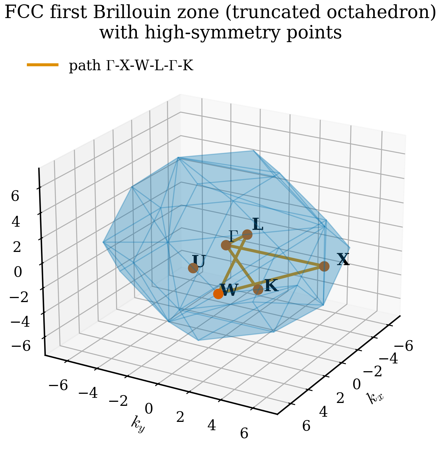
The first BZ for a simple cubic lattice is a cube of edge \(2\pi/a\) centred on the origin. The first BZ for FCC is the truncated octahedron (a truncated octahedron made of six square and eight hexagonal faces) — because the reciprocal lattice of FCC is BCC, the BZ inherits BCC's Wigner–Seitz shape. For BCC, the first BZ is the rhombic dodecahedron.
High-symmetry points
The Brillouin zone has special points where its symmetry is highest. These get conventional names — derived in part from group theory, in part from historical accident — and they are where band structures are evaluated. For FCC (whose BZ is the truncated octahedron), the high-symmetry points are:
- \(\boldsymbol{\Gamma} = (0, 0, 0)\) — the centre of the BZ. Every BZ has a \(\Gamma\) point.
- \(\mathrm{X} = (2\pi/a)(1, 0, 0)\) — centre of a square face (one of six).
- \(\mathrm{L} = (2\pi/a)(1/2, 1/2, 1/2)\) — centre of a hexagonal face (one of eight).
- \(\mathrm{K} = (2\pi/a)(3/4, 3/4, 0)\) — centre of an edge between two hexagonal faces.
- \(\mathrm{W} = (2\pi/a)(1, 1/2, 0)\) — vertex of the BZ.
- \(\mathrm{U} = (2\pi/a)(1, 1/4, 1/4)\) — middle of an edge between a square and hexagonal face.
The canonical band-structure path for FCC materials is \(\Gamma \to \mathrm{X} \to \mathrm{W} \to \mathrm{L} \to \Gamma \to \mathrm{K}\), or some variant.
For BCC the relevant high-symmetry points are \(\Gamma\), \(\mathrm{H}\), \(\mathrm{N}\), \(\mathrm{P}\). For hexagonal lattices: \(\Gamma\), \(\mathrm{M}\), \(\mathrm{K}\), \(\mathrm{A}\), \(\mathrm{L}\), \(\mathrm{H}\). The conventions are tabulated in standard references (Bradley and Cracknell; Setyawan and Curtarolo provide a modern compilation). Codes such as pymatgen and ASE compute the standard paths automatically:
from ase.build import bulk

si = bulk("Si")
path = si.cell.bandpath("LGXWKL", npoints=100)
print(path)            # describes the path
print(path.kpts[:5])   # first five k-points along the path
Pause and recall
Before reading on, try to answer these from memory:
- Write down the defining condition \(\mathbf{b}_i \cdot \mathbf{a}_j = 2\pi\,\delta_{ij}\) and explain in words what it guarantees about \(e^{i\mathbf{G}\cdot\mathbf{r}}\).
- What is the reciprocal lattice of FCC, and what is the shape of the corresponding first Brillouin zone?
- Why is the first Brillouin zone defined as the Wigner–Seitz cell of the reciprocal lattice rather than any other primitive cell?
If any of these is shaky, re-read the preceding section before continuing.
Why band-structure paths are one-dimensional
The electronic eigenvalues of a crystal are functions of the three-component wavevector \(\mathbf{k}\), defined on the Brillouin zone. So properly, the band structure is a set of three-dimensional surfaces \(E_n(\mathbf{k})\). Plotting these in three dimensions is impractical, so the convention is to project them onto a one-dimensional path that connects the high-symmetry points where the dispersion has interesting features. This path is what a typical band-structure plot shows along the horizontal axis.
The choice of path is a convention. Different choices reveal different features. The conventional FCC path \(\Gamma \to \mathrm{X} \to \mathrm{W} \to \mathrm{L} \to \Gamma \to \mathrm{K}\) traverses all the high-symmetry points and is enough to characterise gaps and effective masses.
Bloch's theorem in preview
The reason reciprocal space matters for electronic structure is Bloch's theorem: the eigenstates of a single electron in a periodic potential can be written as
where \(u_{n\mathbf{k}}(\mathbf{r})\) has the same periodicity as the lattice. The wavevector \(\mathbf{k}\) labels a continuous family of eigenstates; the band index \(n\) labels the discrete bands at each \(\mathbf{k}\). Wavevectors differing by a reciprocal-lattice vector \(\mathbf{G}\) give physically equivalent states, so it is enough to consider \(\mathbf{k}\) in the first Brillouin zone.
We will derive Bloch's theorem properly in Chapter 4. For now, take it as the statement that the natural quantum number for an electron in a crystal is a vector in the first Brillouin zone, and that the band structure plots energy versus this vector.
Reciprocal space and momentum
What does \(\mathbf{k}\) mean physically? In free space, \(\hbar \mathbf{k}\) is the momentum of a plane-wave electron. In a crystal, \(\hbar \mathbf{k}\) is the crystal momentum — a quantity that is conserved up to reciprocal-lattice vectors (because the symmetry of the system is translation by \(\mathbf{R}\), not arbitrary translation). The distinction matters when computing transitions: photons carry essentially no crystal momentum, so optical transitions in a band structure are vertical (same \(\mathbf{k}\) initial and final). Phonons can carry crystal momentum, so phonon-assisted transitions are not vertical. This is why indirect-gap semiconductors are poor light absorbers and emitters.
k-point meshes
For practical DFT and MD-on-an-MLIP calculations, we usually do not care about \(E_n(\mathbf{k})\) along a one-dimensional path. We care about integrals over the Brillouin zone — total energy, density, density of states. These integrals are approximated by sums over a discrete set of \(\mathbf{k}\)-points, the k-point mesh or k-mesh.
The standard scheme is the Monkhorst–Pack mesh, which places \(\mathbf{k}\)-points on a regular grid in reciprocal space. A \(4 \times 4 \times 4\) Monkhorst–Pack mesh in a cubic cell has 64 \(\mathbf{k}\)-points (reduced to a smaller number by symmetry). The required density of \(\mathbf{k}\)-points depends on the system: metals need denser meshes than insulators because the Fermi surface is sharp; large unit cells need sparser meshes (their Brillouin zones are smaller, so fewer points are needed to sample them equivalently); small unit cells need denser meshes.
A useful rule of thumb: the product of the number of \(\mathbf{k}\)-points along each direction times the lattice parameter along that direction should be approximately constant. So a \(4 \times 4 \times 4\) mesh for an 8 Å cell becomes a \(2 \times 2 \times 2\) mesh for a 16 Å cell (e.g., after doubling the cell).
from ase.build import bulk
from ase.dft.kpoints import monkhorst_pack

si = bulk("Si")
kpts = monkhorst_pack((4, 4, 4))
print(f"4 x 4 x 4 grid: {len(kpts)} k-points before symmetry reduction")
After symmetry reduction by the space group, a \(4 \times 4 \times 4\) mesh for diamond silicon reduces to 8 irreducible k-points — a dramatic saving that makes the calculation feasible.
We will return to k-point convergence in Chapter 6.
Diffraction and the structure factor
Reciprocal space is also the natural setting for X-ray and neutron diffraction. The intensity of a scattered beam at wavevector \(\mathbf{q}\) is proportional to the modulus squared of the structure factor
where the sum is over atoms in the unit cell, \(f_j\) is the atomic scattering factor (a function of atomic number and \(\mathbf{q}\)), and \(\mathbf{r}_j\) is the atomic position. The condition for constructive interference — Bragg's law — is that \(\mathbf{q}\) equals a reciprocal-lattice vector \(\mathbf{G}\). Diffraction peaks therefore appear at the points of the reciprocal lattice, with intensities set by the structure factor. The systematic absences of certain reflections in particular structures (e.g., the disappearance of \((100)\) in FCC because of the face-centring) are a structure-factor effect.
This is the bridge between simulation and experiment: a crystal we have built in ASE has predictable diffraction peak positions and intensities, and these can be compared directly with X-ray data.
A simple visualisation
To get a feel for the first Brillouin zone, you can plot the BZ boundary together with the high-symmetry path. ASE provides utilities, but the conceptual picture is the one to internalise.
import numpy as np
import matplotlib.pyplot as plt
from ase.build import bulk

si = bulk("Si")
bz = si.cell.bandpath().free_electron_band_structure()  # toy bands

bz_path = si.cell.bandpath("LGXWKL", npoints=200)
print("Special points on this path:", bz_path.special_points)
print("Path:", bz_path.path)
Run this and inspect the special points: \(\Gamma\), X, L, W, K. They are the bookmarks for everything that follows. When you read a band-structure plot, you are walking along this set of bookmarks.
Reciprocal space for phonons
Everything we have said about electrons applies to phonons (lattice vibrations) as well. Each phonon mode is labelled by a wavevector \(\mathbf{q}\) in the first Brillouin zone and a band index. Phonon dispersion plots — \(\omega(\mathbf{q})\) along a one-dimensional path — look structurally identical to electronic band structures, with frequency on the vertical axis. Phonon \(\mathbf{q}\)-meshes are needed for thermodynamic integrals.
The unifying picture: any wave-like excitation in a periodic crystal — electrons, phonons, magnons, plasmons — lives in the same reciprocal space, on the same Brillouin zone, and is labelled by a wavevector in that zone. This is one of the deep unifications that the abstract reciprocal-space machinery delivers.
Common confusions
A handful of stumbling blocks deserve flagging.
The \(2\pi\) factor. Some references (physics convention) define the reciprocal lattice with the \(2\pi\); some (crystallography convention) omit it. ASE's cell.reciprocal() historically omits it; pymatgen uses \(2\pi\). Always check the definition before quoting a value.
Primitive versus conventional cells in reciprocal space. The reciprocal lattice is defined from the primitive direct-lattice vectors. If you start from the conventional cell of an FCC crystal (a cube), naive computation gives you the reciprocal of a cube (another cube), which is the Brillouin zone of a simple-cubic crystal with four-atom basis, not the BCC-shaped FCC Brillouin zone. This causes endless confusion with k-point meshes. When in doubt, work in the primitive cell.
k-points as labels, not particles. A k-point is not a place an electron is; it is a label for a single-particle eigenstate, like a quantum number. Saying the electron is at the X point is a sloppy shorthand for the electron is in the eigenstate of crystal momentum \(\hbar \mathbf{k}_X\).
Path conventions. Different sources use different paths through the BZ for the same structure. X–U–K–\(\Gamma\) and X–W–K–\(\Gamma\) are both legitimate FCC paths. When reproducing a published band structure, check which path was used.
What to memorise
The minimum you should know without thinking: - \(\mathbf{b}_i \cdot \mathbf{a}_j = 2\pi \delta_{ij}\) defines the reciprocal lattice. - The reciprocal of FCC is BCC; of BCC is FCC; of simple cubic is simple cubic; of hexagonal is hexagonal. - \(\Gamma\) is the BZ centre; X is the centre of a square face of the FCC BZ; L is the centre of a hexagonal face. - Bloch states are labelled by \(\mathbf{k}\) in the first BZ and a band index. - Optical transitions are vertical in \(\mathbf{k}\); phonon-assisted transitions are not.
Where this leaves us
We can now describe a crystal in real space (Bravais lattice + basis), build it in code (ase.build.bulk), and describe its dual in reciprocal space (reciprocal-lattice vectors, Brillouin zone, high-symmetry points, k-meshes). This is the structural vocabulary of every electronic-structure method in the rest of the book. Chapter 4 will populate the band structure with electrons; Chapter 5 will compute it self-consistently with DFT.
Before moving on, work through the exercises. They include both pen-and-paper questions and short coding tasks that will cement the geometric intuition this chapter has built.