7.6 Analysing Trajectories¶
Why this section exists
Running an MD simulation generates terabytes of position data. The physics is not in the raw data; it is in time- and ensemble-averages computed from it. A trajectory file is a sequence of snapshots; an observable is what you compute by integrating or correlating over the sequence. Every connection between simulation and experiment goes through this layer.
The picture: you have a movie of atoms wiggling. You want to extract numbers — the diffusion coefficient, the radial distribution function, the phonon spectrum — that an experimentalist can measure. Each of these is a specific functional of the trajectory. This section spells out the functionals and their estimators.
Definition 7.6.1 (Trajectory). A trajectory is a sequence \(\{(\mathbf{r}^n_i,\mathbf{v}^n_i)\}_{n=0}^{N_t-1}\) for \(i=1,\ldots,N\) atoms, sampled at times \(t_n = n\Delta t_\mathrm{save}\) with frame interval \(\Delta t_\mathrm{save}\) a multiple of the MD timestep.
scripts/figures/fig_rdf_real.py; a simpler analytic-curve illustration is in scripts/figures/fig_rdf_phases.py.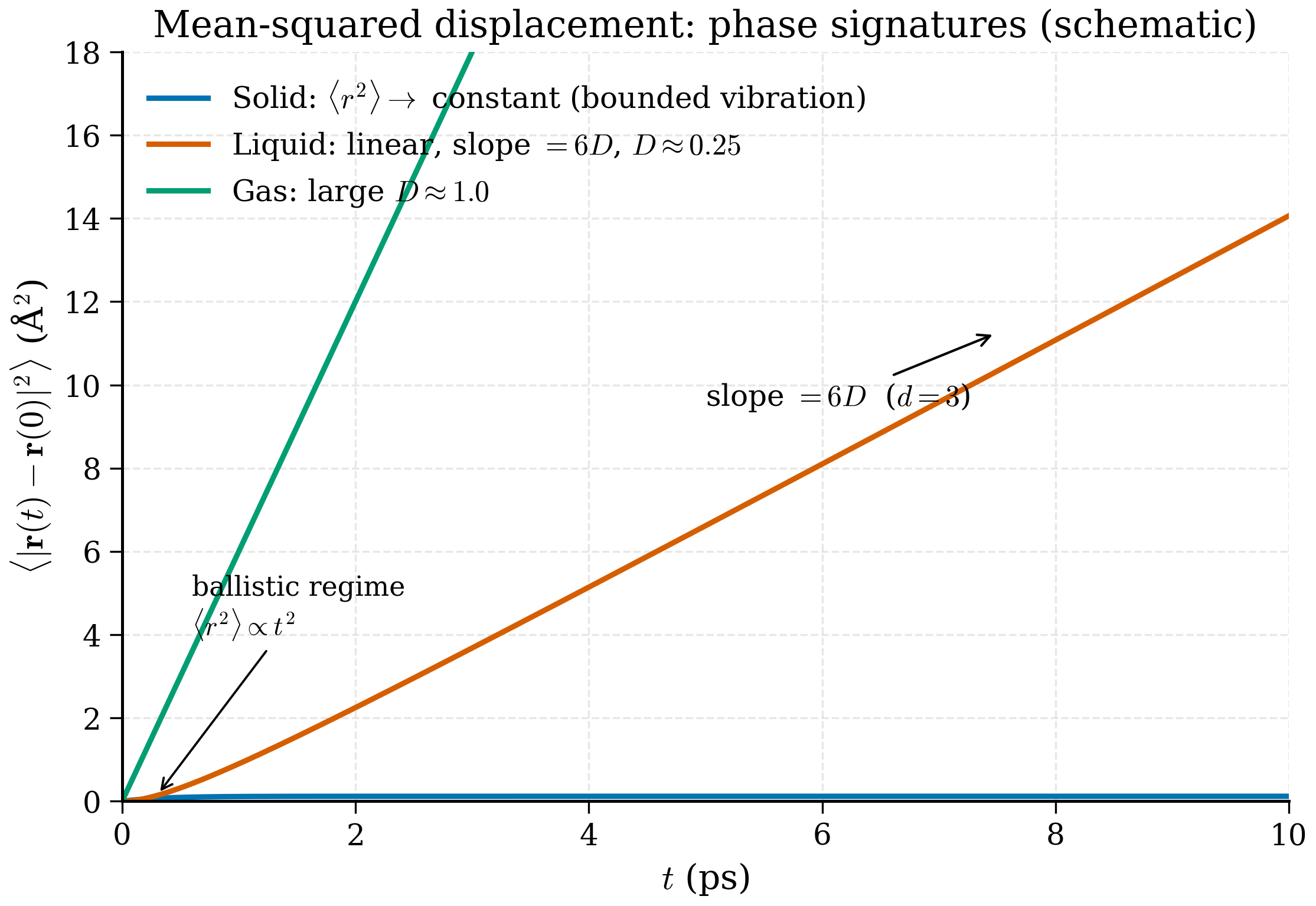
A LAMMPS trajectory is a few megabytes to a few terabytes of \((x, y, z)\) data. The physics is not in the data; it is in the time- and ensemble-averages you compute from it. This section covers the standard analyses: mean squared displacement (transport), radial distribution function (structure), velocity autocorrelation function (vibrations), and structure factor (the same structure, in reciprocal space). We code MSD and \(g(r)\) from scratch with NumPy, then compare against MDAnalysis as a sanity check.
Mean squared displacement¶
Key idea (Einstein relation)
A diffusing atom's mean-squared displacement grows linearly with time, with slope \(2dD\) where \(d\) is the dimensionality and \(D\) the diffusion coefficient. The Einstein relation \(D = \mathrm{MSD}(t)/(2dt)\) is the practical way to extract \(D\) from an MD trajectory. The linear regime starts after the ballistic regime (typically picoseconds) and ends before statistical noise dominates (typically when \(t\) approaches a fraction of the simulation length).
The MSD of a single atom is the time-averaged squared distance from its initial position:
where the average is over starting times \(t_0\) and over atoms of the relevant species. For a free Brownian particle in \(d\) dimensions the MSD grows as \(2 d D t\):
so the diffusion coefficient is
This is the Einstein relation.
Deriving Einstein's relation
Take the Langevin equation in the overdamped limit (large \(\gamma\), where momentum relaxes fast and only position diffuses): \(\gamma m\dot{\mathbf{r}} = \boldsymbol{\eta}(t)\) with \(\langle\eta_\alpha(t)\eta_\beta(t')\rangle = 2m\gamma k_BT\,\delta_{\alpha\beta}\delta(t-t')\). Integrating from 0 to \(t\): $\(\mathbf{r}(t) - \mathbf{r}(0) = \frac{1}{\gamma m}\int_0^t \boldsymbol{\eta}(t')\,dt'.\)$ Squaring and ensemble-averaging: $\(\langle|\mathbf{r}(t)-\mathbf{r}(0)|^2\rangle = \frac{1}{\gamma^2 m^2}\int_0^t\int_0^t \langle\boldsymbol{\eta}(t')\cdot\boldsymbol{\eta}(t'')\rangle\,dt'\,dt'' = \frac{1}{\gamma^2 m^2}\cdot d\cdot 2m\gamma k_BT\cdot t = \frac{2d k_BT}{m\gamma}\,t.\)$ Comparing to \(\mathrm{MSD}(t) = 2dD t\) gives \(D = k_BT/(m\gamma)\), the Stokes-Einstein form. In an MD simulation without an explicit friction, \(D\) is determined by the effective friction from interatomic collisions; the relation \(\mathrm{MSD} = 2dD t\) still holds in the long-time limit, and \(D\) is what you extract from the slope.
The factor \(d\) (dimensionality) is important: a Cartesian-x-only MSD grows as \(2Dt\), a 3D MSD as \(6Dt\), a 2D-slab MSD as \(4Dt\). Be careful which one your analysis function returns. It is the standard way to extract \(D\) from an MD trajectory.
Pause and recall
Before reading on, try to answer these from memory:
- State the Einstein relation and explain how the diffusion coefficient \(D\) is extracted from the slope of the mean-squared displacement.
- Why does the dimensionality factor \(d\) matter — what slope would you expect for a 3D MSD versus a Cartesian-x-only MSD?
- Why must you use unwrapped coordinates for the MSD, and what does the MSD of a solid look like versus that of a liquid?
If any of these is shaky, re-read the preceding section before continuing.
Two practical considerations:
- Use unwrapped coordinates (see §7.2). Wrapped MSD saturates at \(L^2/4\), garbage.
- Use a time-origin average. A naive evaluation of (7.51) uses only \(\mathbf{r}(0)\) as the reference; averaging over many starting times reduces variance dramatically. For a trajectory of length \(T\), the time-origin-averaged MSD at lag \(\tau\) is
$$ \mathrm{MSD}(\tau) = \frac{1}{T - \tau} \int_0^{T - \tau} |\mathbf{r}(t + \tau) - \mathbf{r}(t)|^2\, dt. \tag{7.54} $$
A NumPy implementation, operating on an (n_frames, n_atoms, 3) array of unwrapped positions:
"""Mean squared displacement from a trajectory.

Time-origin-averaged Einstein-relation MSD.
"""
from __future__ import annotations
import numpy as np


def msd(positions: np.ndarray) -> np.ndarray:
    """Compute the time-origin-averaged MSD of a trajectory.

    Parameters
    ----------
    positions : (n_frames, n_atoms, 3) array of unwrapped positions.

    Returns
    -------
    (n_frames,) array of MSD values at each lag in frames.
    """
    n_frames, n_atoms, _ = positions.shape
    msd_out = np.zeros(n_frames, dtype=np.float64)
    for tau in range(n_frames):
        diffs = positions[tau:] - positions[:n_frames - tau]
        msd_out[tau] = np.mean(np.sum(diffs ** 2, axis=-1))
    return msd_out
This is \(O(N_\mathrm{frames}^2 N_\mathrm{atoms})\) — fine for \(10^4\) frames, slow for \(10^6\). A FFT-based version (Welford's trick or the auto-correlation theorem) reduces it to \(O(N_\mathrm{frames} \log N_\mathrm{frames} \cdot N_\mathrm{atoms})\) and is what MDAnalysis and tidynamics use internally.
Extracting \(D\) from the resulting MSD curve: plot \(\mathrm{MSD}(t)\) vs \(t\), identify the linear regime (typically excluding the first picosecond, where ballistic motion gives MSD \(\propto t^2\), and the last few percent of the trajectory, where statistics are poor), and fit a straight line. The slope divided by 6 is \(D\).
def diffusion_coefficient(t: np.ndarray, msd_t: np.ndarray,
                          fit_range: tuple[float, float]) -> float:
    """Linear fit to MSD in a chosen time range.

    Parameters
    ----------
    t, msd_t : time array and MSD array, same length.
    fit_range : (t_min, t_max) for the linear fit, in same units as t.

    Returns
    -------
    Diffusion coefficient D = slope / 6.
    """
    mask = (t >= fit_range[0]) & (t <= fit_range[1])
    slope, _intercept = np.polyfit(t[mask], msd_t[mask], 1)
    return slope / 6.0
For liquid argon at 100 K with the LJ parameters of §7.5, the expected diffusion coefficient is around \(2 \times 10^{-9}\) m\(^2\)/s. In LAMMPS metal units (Å\(^2\)/ps), \(D = 2 \times 10^{-9}\,\mathrm{m}^2/\mathrm{s} = 0.02\) Å\(^2\)/ps. Verify against this; an order-of-magnitude discrepancy points to wrapped coordinates or a thermostat bug.
Example 7.6.2 (Diffusion of liquid argon at 100 K). Problem. From a 200 ps NVT MD trajectory of 4000 LJ-Ar atoms at 100 K, compute \(D\).
Solution. (i) Unwrap coordinates using image flags. (ii) Compute time-origin-averaged MSD via (7.54). (iii) Identify the linear regime — typically 2-100 ps for this system. (iv) Linear-fit polyfit(t, msd, 1); divide slope by 6.
Expected outcome: \(D \approx 0.02\) Å\(^2\)/ps \(= 2\times 10^{-9}\) m\(^2\)/s, within 10% of the experimental value at the same temperature.
Discussion. The ballistic regime (\(t<1\) ps) has MSD \(\propto t^2\) — exclude it from the fit. The very late regime (last 10% of the trajectory) has poor statistics (few independent time origins) — exclude it too. The intermediate "diffusive" regime is where Einstein's relation holds.
Radial distribution function¶
Key idea (Radial distribution function)
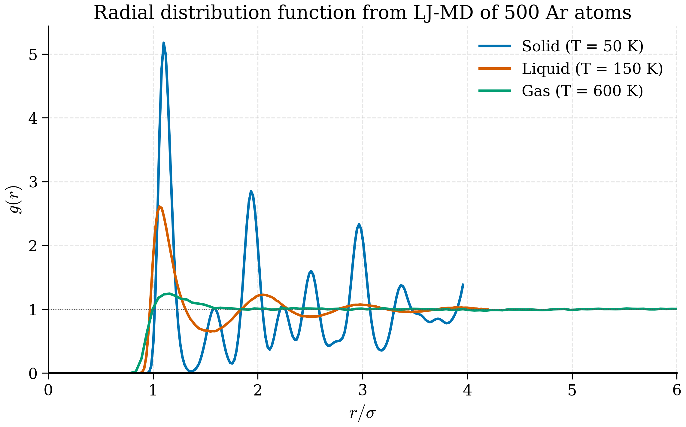
The RDF \(g(r)\) counts pair distances normalised to the ideal-gas expectation. Crystal: sharp peaks at neighbour-shell distances. Liquid: broad first peak, smaller secondary peaks decaying to 1. Gas: nearly flat at 1 with a dip below contact. \(g(r)\) is the most direct probe of local structure and connects to X-ray and neutron scattering through Fourier transform.
The radial distribution function \(g(r)\) measures the conditional probability of finding another atom at distance \(r\) from a reference atom, normalised by what would be expected in an ideal gas at the same density:
Deriving the practical histogram form
To turn (7.55) into an algorithm, replace the continuous \(\delta(r-r_{ij})\) by a histogram bin of width \(\Delta r\). The number of pairs falling into the spherical shell of inner radius \(r\) and outer radius \(r+\Delta r\) is
$\(n_\mathrm{shell}(r) = \frac{1}{N_\mathrm{frames}}\sum_\mathrm{frames}\sum_{i<j}\mathbb{1}[r \le r_{ij} < r+\Delta r],\)$
where the indicator function counts pairs in the shell. The expected number for an ideal gas at density \(\rho = N/V\) would be
$\(n_\mathrm{ideal}(r) = N\cdot\rho\cdot 4\pi r^2\,\Delta r / 2,\)$
where the factor of \(N\rho\) is the pair count, the \(4\pi r^2\,\Delta r\) is the shell volume, and the \(1/2\) avoids double-counting. The radial distribution function is the ratio:
$\(g(r) = \frac{n_\mathrm{shell}(r)}{n_\mathrm{ideal}(r)} = \frac{2\,n_\mathrm{shell}(r)}{N\,\rho\,4\pi r^2\,\Delta r}.\)$
This is exactly what the rdf function below computes, with \(n_\mathrm{shell}(r)\) accumulated as hist[idx] and the normalisation
$\(\mathrm{norm}(r) = \rho\,4\pi r^2\,\Delta r\,\frac{N}{2}\cdot N_\mathrm{frames}.\)$
Forgetting the \(4\pi r^2\) shell-volume normalisation is the most common bug in homegrown \(g(r)\) implementations — the resulting curve looks vaguely like an RDF but with the wrong shape near \(r=0\) and a non-converging tail.
In a perfect crystal \(g(r)\) is a series of sharp delta functions at the discrete neighbour distances. In a liquid the first peak is broad and rounded — typically near \(r/\sigma \approx 1\) for LJ — with smaller, broader peaks at successive shells that decay to \(g(r) \to 1\) as \(r \to \infty\). In a dilute gas \(g(r) \approx 1\) everywhere except a small dip below 1 inside the contact distance.
Practical computation: bin the pair distances over a trajectory and normalise by the shell volume.
def rdf(positions: np.ndarray, box: np.ndarray,
        r_max: float, n_bins: int = 200) -> tuple[np.ndarray, np.ndarray]:
    """Radial distribution function from a trajectory.

    Parameters
    ----------
    positions : (n_frames, n_atoms, 3), wrapped or unwrapped.
    box : (3,) orthorhombic box dimensions, assumed constant.
    r_max : maximum distance; must be < min(box) / 2.
    n_bins : number of histogram bins.

    Returns
    -------
    r : (n_bins,) bin centres.
    g : (n_bins,) radial distribution function.
    """
    n_frames, n_atoms, _ = positions.shape
    rho = n_atoms / np.prod(box)            # number density
    dr = r_max / n_bins
    hist = np.zeros(n_bins, dtype=np.int64)

    for frame in positions:
        for i in range(n_atoms - 1):
            dvec = frame[i + 1:] - frame[i]            # broadcast
            dvec -= box * np.round(dvec / box)          # min image
            d = np.linalg.norm(dvec, axis=-1)
            d = d[d < r_max]
            idx = (d / dr).astype(np.int64)
            np.add.at(hist, idx, 1)

    # Normalisation: shell volume 4πr^2 dr times density times pairs
    r = (np.arange(n_bins) + 0.5) * dr
    shell_vol = 4 * np.pi * r ** 2 * dr
    norm = shell_vol * rho * n_atoms * n_frames / 2.0   # /2 for i<j pairs counted once
    g = hist / norm
    return r, g
A few subtleties:
- We loop over \(i\) and consider only \(j > i\) to count pairs once, then divide by 2 in the normalisation. Equivalently, you could loop over all \(i \ne j\) and divide by \(N \cdot N_\mathrm{frames}\).
- \(r_\mathrm{max}\) must be less than half the smallest box dimension; otherwise atoms within \(r_\mathrm{max}\) in two images appear, double-counting.
- For binary systems, you compute three RDFs: \(g_{AA}\), \(g_{AB}\), \(g_{BB}\). The normalisation prefactor changes accordingly: \(\rho_B\) for the AB pair sums.
The first peak position of \(g(r)\) in a liquid is the typical nearest-neighbour distance; the peak height is a coordination-shell signature (\(\sim 3\) for liquid argon, \(\sim 2.5\) for water O-O). The integral up to the first minimum gives the coordination number,
which for liquid Ar is about 11 (compared to 12 in the fcc crystal).
Velocity autocorrelation function and VDOS¶
The velocity autocorrelation function (VACF),
measures how strongly an atom's velocity at time \(t\) correlates with its velocity at \(t = 0\). For a free particle \(C_{vv}(t) = 1\) always; for an oscillator \(C_{vv}(t) = \cos(\omega t)\); for a damped oscillator, a decaying cosine; for a liquid, a positive peak at zero followed by a negative dip (caging by neighbours) and decay.
The Fourier transform of \(C_{vv}\) is the vibrational density of states (VDOS):
Why FFT of VACF gives VDOS — Wiener-Khinchin
The Wiener-Khinchin theorem states that the power spectral density of a stationary stochastic process equals the Fourier transform of its autocorrelation function. For atomic velocities: $\(|\tilde{\mathbf{v}}(\omega)|^2 = \int_{-\infty}^\infty C_{vv}(t)\,e^{-i\omega t}\,dt,\)$ where \(\tilde{\mathbf{v}}(\omega)\) is the Fourier transform of \(\mathbf{v}(t)\) over a long trajectory. The left-hand side is the power spectrum — how much kinetic energy lives at each frequency. The right-hand side is the FFT of the VACF.
For a harmonic crystal, kinetic energy is shared equally between all normal modes (equipartition), so the power spectrum is a sum of delta functions at each phonon frequency, weighted by mode multiplicity. Integrated, this is the phonon density of states. In a real MD simulation the deltas are broadened by the finite simulation time (the energy resolution is \(\Delta\omega \sim 2\pi/T_\mathrm{sim}\)) and by anharmonicity, but the positions of dominant peaks still correspond to phonon branches.
In a liquid, the modes are not propagating but the VDOS still encodes characteristic vibrational frequencies — the low-frequency end gives transport-related modes (related to the diffusion coefficient by \(D = \tfrac{1}{3}\int_0^\infty C_{vv}(t)\,dt\), another consequence of Green-Kubo) and the high-frequency end gives the local-cage rattling.
For a harmonic crystal, VDOS reduces to the phonon density of states; peaks correspond to optical branches, the low-frequency \(\omega^2\) behaviour to acoustic phonons. For a liquid, the spectrum is broadened — there are no propagating modes — but the position of dominant features still reflects the underlying short-range bonding.
Implementation parallels MSD: a time-origin-averaged correlation, then FFT.
def vacf_and_vdos(
    velocities: np.ndarray, dt: float
) -> tuple[np.ndarray, np.ndarray, np.ndarray]:
    """Velocity autocorrelation and vibrational DOS.

    Parameters
    ----------
    velocities : (n_frames, n_atoms, 3).
    dt : time step between frames.

    Returns
    -------
    t, C(t), VDOS(omega)
    """
    n_frames, n_atoms, _ = velocities.shape
    v_flat = velocities.reshape(n_frames, -1)           # (T, 3N)
    # Use FFT-based autocorrelation
    F = np.fft.rfft(v_flat, axis=0, n=2 * n_frames)
    acf = np.fft.irfft(F * np.conj(F), axis=0)[:n_frames]
    acf = acf.sum(axis=1)
    norm = (n_frames - np.arange(n_frames)) * v_flat.shape[1]
    acf = acf / norm
    acf /= acf[0]
    t = np.arange(n_frames) * dt
    # VDOS by FFT
    vdos = np.abs(np.fft.rfft(acf))
    omega = 2 * np.pi * np.fft.rfftfreq(n_frames, d=dt)
    return t, acf, vdos
Structure factor¶
The static structure factor \(S(q)\) is the Fourier transform of the radial distribution function:
or equivalently the squared magnitude of the density Fourier component,
\(S(q)\) is what X-ray scattering, neutron scattering, and total-scattering experiments directly measure. Comparing simulation \(S(q)\) to experimental \(S(q)\) is the gold-standard validation of a force field for liquids and amorphous solids.
For a crystal, \(S(q)\) shows sharp Bragg peaks at reciprocal lattice vectors. For a liquid, broad peaks; the first peak position \(q_1 \approx 2\pi/r_1\) where \(r_1\) is the first \(g(r)\) maximum.
Computing \(S(q)\) from a trajectory¶
Two practical routes. Direct (7.60):
def structure_factor_direct(positions: np.ndarray, q_vectors: np.ndarray) -> np.ndarray:
    """S(q) by direct evaluation of |sum exp(i q·r)|^2 / N."""
    n_frames, n_atoms, _ = positions.shape
    n_q = q_vectors.shape[0]
    S = np.zeros(n_q, dtype=np.float64)
    for frame in positions:
        phases = q_vectors @ frame.T            # (n_q, n_atoms)
        rho_q = np.exp(1j * phases).sum(axis=1) # (n_q,)
        S += np.abs(rho_q) ** 2 / n_atoms
    return S / n_frames
Indirect via \(g(r)\) Fourier transform: $\(S(q) = 1 + 4\pi\rho\,\int_0^\infty [g(r)-1]\,\frac{\sin(qr)}{qr}\,r^2\,dr.\)$ This is the angular-averaged version of (7.59); it converts your already-computed \(g(r)\) to \(S(q)\) with one integral per \(q\).
Both routes should agree to within statistics. Discrepancies often indicate that \(g(r)\) was not computed out to a large enough \(r_\mathrm{max}\) (truncation introduces ringing in \(S(q)\) at high \(q\)) or that the trajectory is too short to converge the structure factor at long wavelengths.
Coordination number and bond-orientational order¶
Beyond the simple \(g(r)\) peak count, two derived quantities matter for understanding local structure.
Coordination number¶
Given a cutoff \(r_c\) chosen as the first minimum of \(g(r)\), the coordination number of atom \(i\) is $\(Z_i = \sum_{j\ne i} \mathbb{1}[r_{ij} < r_c],\)$ and the average coordination \(\langle Z\rangle\) characterises the structure. For liquid Ar at 100 K, \(\langle Z\rangle \approx 11\); for fcc Ar at 50 K, exactly 12. The distribution of \(Z_i\) across atoms is sometimes more informative than the mean: a bimodal distribution indicates phase coexistence or local order parameter heterogeneity.
Steinhardt \(Q_l\) parameters¶
For distinguishing crystal structures (fcc vs bcc vs hcp vs liquid), Steinhardt-Nelson-Ronchetti bond-orientational order parameters are the standard. Define the local bond order for atom \(i\): $\(Q_{lm}(i) = \frac{1}{Z_i}\sum_{j\in\mathrm{neighbours}(i)} Y_{lm}(\theta_{ij}, \phi_{ij}),\)$ where \(Y_{lm}\) are spherical harmonics and \((\theta_{ij}, \phi_{ij})\) are the polar angles of the bond vector. The rotationally-invariant magnitude $\(Q_l(i) = \sqrt{\frac{4\pi}{2l+1}\sum_{m=-l}^l |Q_{lm}(i)|^2}\)$ takes characteristic values for ideal crystals: \(Q_6 = 0.575\) for fcc, \(Q_6 = 0.628\) for bcc, \(Q_6 \approx 0.485\) for hcp, \(Q_6 \approx 0.3\) for liquid. Plotting \(Q_4\) vs \(Q_6\) for every atom gives a 2D scatter that cleanly separates crystal phases — the Steinhardt parameter is the work-horse order parameter for nucleation studies.
Green-Kubo transport coefficients¶
The Einstein relation gives diffusion via \(\mathrm{MSD}\to 6Dt\). The same idea applies to any transport coefficient through a Green-Kubo formula: the integral of an autocorrelation function gives a transport coefficient. The most useful are:
Diffusion (Green-Kubo form): $\(D = \frac{1}{3}\int_0^\infty C_{vv}(t)\,dt,\)$ which can be computed from the VACF and gives the same answer as the Einstein relation in principle, often faster in practice for short trajectories.
Shear viscosity:
$\(\eta = \frac{V}{k_BT}\int_0^\infty \langle \sigma_{xy}(0)\sigma_{xy}(t)\rangle\,dt,\)$
where \(\sigma_{xy}\) is the off-diagonal stress tensor. LAMMPS' compute pressure gives the instantaneous stress; the Green-Kubo integral converges slowly (long tails from collective modes) and typically needs nanosecond trajectories with high sampling rate.
Thermal conductivity: $\(\kappa = \frac{V}{k_BT^2}\int_0^\infty \langle \mathbf{J}_E(0)\cdot\mathbf{J}_E(t)\rangle\,dt,\)$ with \(\mathbf{J}_E\) the energy current. Hardest to converge; nanoseconds at fine sampling.
The trade-off with Green-Kubo is that the integral has a long tail: cutting it off too early biases the coefficient. A common practical rule is to integrate until the autocorrelation has decayed to ~1% of its initial value, but for hydrodynamically slow modes this may require integrating much further. Non-equilibrium MD (NEMD), where you apply a fictitious driving force and measure the steady-state response, is often more efficient for shear viscosity in particular; LAMMPS' fix viscosity and fix nvt/sllod implement this.
ASE Trajectory and MDAnalysis¶
The reference analyses above are fine for small trajectories. For production work, two libraries do this better:
ASE reads LAMMPS dump files and many other formats:
from ase.io import read
traj = read("argon.lammpstrj", index=":")       # list of Atoms
positions = np.array([a.get_positions() for a in traj])
box = np.array(traj[0].cell.lengths())
MDAnalysis is a more capable framework specifically for trajectory analysis:
import MDAnalysis as mda
from MDAnalysis.analysis import rdf, msd

u = mda.Universe("argon.lammpstrj", topology_format="LAMMPSDUMP",
                 format="LAMMPSDUMP")

# RDF
g_calc = rdf.InterRDF(u.atoms, u.atoms, nbins=200, range=(0.5, 10.0))
g_calc.run()
r = g_calc.results.bins
g = g_calc.results.rdf

# MSD with FFT
msd_calc = msd.EinsteinMSD(u, select="all", msd_type="xyz", fft=True)
msd_calc.run()
times = msd_calc.times
msd_t = msd_calc.results.timeseries
MDAnalysis handles wrapping, unwrapping, image flags, mixed-species selections, FFT-based autocorrelations, and all the bookkeeping that becomes tedious in pure NumPy for large trajectories. For anything beyond the simplest analyses, prefer it.
That said, knowing how the algorithms work — what (7.51), (7.55), (7.57) really mean as estimators — is essential. The libraries are fast at the wrong analysis just as cheerfully as at the right one.
Sanity-check your analysis on a known system
A 10 ps trajectory of an ideal gas at temperature \(T\) should give \(D = \infty\) (diverging MSD), \(g(r) = 1\) for all \(r > 0\), and \(C_{vv}(t) = \delta_{t,0}\) in the free-particle limit. Running your analysis pipeline on such a synthetic trajectory catches index errors and normalisation bugs before they corrupt research results.
Error estimates: block averaging¶
Every quantity you compute from an MD trajectory comes with statistical error. Ignoring it is the single most common reason for mismatch between simulation and experiment that is not a force-field problem.
Naive standard error of the mean assumes independent samples: \(\sigma_\mu = \sigma/\sqrt{N}\). MD samples are correlated — successive frames are dynamically related — so this underestimates the error by a factor proportional to the autocorrelation time.
Block averaging is the standard cure. Partition the trajectory into \(B\) contiguous blocks; compute the mean of each block; the variance of these block means, divided by \(B-1\), is an unbiased estimator of the error of the overall mean. As \(B\) decreases (blocks get longer), the block means become more nearly independent and the error estimate converges to its asymptotic value. Plotting the estimated error vs block size and looking for a plateau is the diagnostic.
def block_average(samples: np.ndarray, n_blocks: int) -> tuple[float, float]:
    """Block-averaged mean and standard error."""
    block_size = len(samples) // n_blocks
    block_means = np.array([samples[i*block_size:(i+1)*block_size].mean()
                             for i in range(n_blocks)])
    mean = block_means.mean()
    sem = block_means.std(ddof=1) / np.sqrt(n_blocks)
    return mean, sem
A useful exercise: compute the temperature of an NVE simulation and check the error bar. For \(N = 1000\) atoms over 100 ps with \(\Delta t = 1\) fs, you have \(10^5\) frames. The intrinsic temperature fluctuation is \(T\sqrt{2/(3N)} \approx 2.6\) K at 100 K. The autocorrelation time of \(T_\mathrm{kin}\) is the inverse of the lowest phonon frequency, \(\sim 1\) ps, so the effective number of independent samples is 100. The standard error of the mean \(T\) is therefore \(2.6/\sqrt{100} = 0.26\) K — not 0.008 K as naive \(\sqrt{N}\) would suggest. Quoting \(T\) to 0.01 K from a 100 ps simulation is overconfident by a factor of 30.
Section summary¶
The four standard MD analyses, with what each measures and the experiment it connects to:
- MSD → diffusion coefficient \(D\) via Einstein's relation \(\mathrm{MSD} = 2dD\,t\). Probes long-time transport. Connects to NMR pulsed-field-gradient experiments, tracer diffusion measurements.
- RDF \(g(r)\) → local structure. Peak positions are typical neighbour distances; integrated first peak is coordination number. Connects to X-ray and neutron diffraction via \(S(q)\).
- VACF $C_{vv}(t) → $ VDOS via Fourier transform. For crystals, the phonon density of states; for liquids, broadened modes. Connects to inelastic neutron scattering, IR spectroscopy.
- Structure factor \(S(q)\) → scattering experiments directly. Bragg peaks for crystals, broad features for liquids. The most direct simulation-experiment comparison.
All four are typically implemented in MDAnalysis, ASE, or tidynamics; the implementations here are pedagogical — to know what the libraries are computing, run your own against theirs once.
Error bars from block averaging are non-negotiable. The factor \(\sqrt{\tau_\mathrm{corr}/T_\mathrm{sim}}\) in the effective sample size is what separates a trustworthy result from a hopeful one.
What we have¶
We can now run an MD simulation and extract from it the structural (\(g(r)\), \(S(q)\)), dynamical (MSD, \(D\), VACF), and thermodynamic (pressure, energy, temperature) observables that connect simulation to experiment. This is enough to complete a typical materials-science MD study end-to-end.
Remark 7.6.3 (Trajectory file formats). LAMMPS' native dump format is text-based and bulky. For production use a binary or compressed format: LAMMPS supports dump dcd, dump xtc, dump nc (NetCDF) — all of these are faster to write, smaller on disk, and readable by MDAnalysis. For ten-nanosecond trajectories of large systems, text-format files can reach hundreds of gigabytes; binary formats compress 10-100×. Switch as soon as you outgrow the example-level workflow.
The next chapter (Chapter 8) tightens the statistical-mechanical underpinnings: which ensemble are we actually sampling, how do we compute free energies, and how do we extract transport coefficients more carefully via Green-Kubo. Chapters 9–11 then return to force fields and replace the classical models of §7.4 with machine-learning potentials trained on DFT.
The exercises (§7.7) practise the integrator, the analyses, and the LAMMPS workflow.